Matrix & Vector Techniques

• 1. Quadratic Form as Matrix Representation
• 2. Diagonal Matrix
• 3. Key Properties of Symmetric Matrices
• 4. Skew-Symmetric Matrix
• 5. Trace Properties
• 6. Determinant Consistency
• 7. Determinant of a Block Matrix
• 8. Area of Polygons
• 9. Rank Properties
• 10. Orthogonal Projection
• 11. Cross Product
• 12. Cayley-Hamilton Theorem
• 13. Transformations
• 14. Jacobian

1. Quadratic Form as Matrix Representation

It is often useful when getting the maximum and minimum of eigenvalues of a diagonal matrix. $$\begin{aligned} a x^2 + 2 b x y + c y^2 &= \left(\begin{array}{cc} x & y \end{array}\right) \left(\begin{array}{cc} a & b \\ c & d \end{array}\right) \left(\begin{array}{c} x \\ y \end{array}\right) \\\\ a x^2 + b y^2 + c z^2 + 2 d x y + 2 e x z + 2 f y z &= \left(\begin{array}{ccc} x & y & z \end{array}\right) \left(\begin{array}{ccc} a & d & e \\ d & b & f \\ e & f & c \end{array}\right) \left(\begin{array}{c} x \\ y \\ z \end{array}\right) \end{aligned}$$

Mainly, the symmetric matrix is used as above, the important note is that the symmetric matrix is not necessary so. Other matrices can be used for this, but the symmetric matrix is convenient since it has useful properties. However, it may occur the symmetric matrix is not available, and in that case, still this form can be derived. More specifically, the general representation is as follows. $$\begin{aligned} a x^2 + b y^2 &+ c z^2 + 2 d x y + 2 e x z + 2 f y z = \left(\begin{array}{ccc} x & y & z \end{array}\right) M \left(\begin{array}{c} x \\ y \\ z \end{array}\right), \quad M = \left(\begin{array}{ccc} m_{11} & m_{12} & m_{13} \\ m_{21} & m_{22} & m_{23} \\ m_{31} & m_{32} & m_{33} \end{array}\right) \end{aligned} \\ \begin{aligned} \implies m_{11} = a, \quad m_{22} = b, \quad m_{33} = c, \quad m_{12} + m_{21} = 2d, \quad m_{13} + m_{31} = 2e, \quad m_{23} + m_{32} = 2f \end{aligned}$$

But, let $A$ be the symmetric matrix from the above representations from now. Consider an eigenvector $v$ and an eigenvalue $\lambda$ of a matrix $A$, which is $Av = \lambda v$. Then, $v^tAv = v^t\lambda v = \lambda v^t v$. Therefore, $$\begin{aligned} \lambda = \cfrac{v^t A v}{v^t v} \end{aligned}$$

Especially, when $\Vert v \Vert = 1$, $\lambda = v^t A v^t$. As such, the maximum and minimum of eigenvalues can be produced from $v^t A v^t$. Meanwhile, as if a quadratic expression can be rotated to remove its cross-terms such as $xy$, the diagonalization of a matrix acts as deleting these cross-terms. From this perspective, the principal axis theorem appears which introduces a transformation of quadratic forms used in the beginning. Let $\lambda_i$ be an eigenvalue of the symmetric matrix $A$. Then, the transformation is as follows. $$\begin{aligned} a x^2 + 2 b x y + c y^2 = k &\implies \lambda_1 x^2 + \lambda_2 y^2 = k \\ a x^2 + b y^2 + c z^2 + 2 d x y + 2 e x z + 2 f y z = k &\implies \lambda_1 x^2 + \lambda_2 y^2 + \lambda_3 z^2 = k \end{aligned}$$

2. Diagonal Matrix

For a matrix $A \in \mathbb{R^{n \times n}}$, $A$ is called diagonalizable if there exists an invertible matrix $P$ and a diagonal matrix $D$ such that $D = P^{-1}AP$. Such $P$ and $D$ are not unique, and $A$ and $D$ are called similar. There are some conditions to be diagonalizable as follows.

• $A$ is symmetric.
• $A$ has $n$ linearly independent eigenvectors.
• $A$ has $n$ different eigenvalues.
• The minimal polynomial consists of distinct linear factors.
• The algebraic multiplicity is equal to the geometric multiplicity.
  • Assume that the characteristic polynomial of $A$ is $f(\lambda) = (\lambda - \alpha)^m(\lambda - \beta) \cdots$ for $1 < m < n$. Although the algebraic multiplicity of $\lambda = \alpha$ is $m$, it shoud be checked if $\dim \ker(A - \alpha I) = m$. Since $\dim \ker (A - \alpha I) + \text{rank}(A - \alpha I) = n$ as mentioned in this note, $A$ is diagonalizable if $n - \text{rank}(A - \alpha I) = m$.

Furthermore, $A$ and $D = P^{-1}AP$ have the following properties in common.

• $\vert A \vert = \vert D \vert$,
• $A$ and $D$ have the same eigenvalues, ranks, and invertibility,
• $A$ and $D$ do not always have the same eigenvectors.

3. Key Properties of Symmetric Matrices

For a symmetric matrix $A \in \mathbb{R^{n \times n}}$, all eigenvalues are real numbers. For example, let $A = \left(\begin{array}{cc} a & b \\ b & c \end{array}\right)$ and $I = \left(\begin{array}{cc} 1 & 0 \\ 0 & 1 \end{array}\right)$. Also, let $\lambda$ is an eigenvalue of $A$. Then, the discriminant $D$ can be obtained as follows. $$\begin{aligned} \vert A - \lambda I \vert &= (a - \lambda)(c - \lambda) - b^2 = \lambda^2 - (a + c)\lambda + ac - b^2 = 0 \\\\ \implies D &= (a + c)^2 - 4(ac - b^2) = (a - c)^2 + 4b^2 \geq 0 \end{aligned}$$

Therefore, all eigenvalues of $A$ are real numbers. Meanwhile, the correspondent eigenvectors for different eigenvalues of $A$ are perpendicular, so $A$ can be diagonalized. Let $v_1$ and $v_2$ be the correspondent eigenvectors for $\lambda_1 \ne \lambda_2$, which means $A v_1 = \lambda_1 v_1$ and $A v_2 = \lambda_2 v_2$. Considering that $x \cdot y = x^t y$ for $x, y \in \mathbb{R^{n \times 1}}$ and $A^t = A$, $$\begin{aligned} \lambda_1 (v_1 \cdot v_2) = (\lambda_1 v_1) \cdot v_2 = Av_1 \cdot v_2 = (v_1^t A^t)v_2 = v_1^t A v_2 = v_1^t (\lambda_2 v_2) = \lambda_2 (v_1^t v_2) = \lambda_2 (v_1 \cdot v_2) \end{aligned}$$

This implies that $(\lambda_1 - \lambda_2)(v_1 \cdot v_2) = 0$. Since $\lambda_1 \ne \lambda_2$, $v_1 \cdot v_2 = 0$. As such, the correspondent eigenvectors are perpendicular. Other key properties can be listed as follows. Let $B$ be also a symmetric matrix. Then, the following statements hold.

• $A^2$, $A^3$, and $A+B$ are also symmetric.

  $(A^2)^t = A^t A^t = AA = A^2$, $\quad (A+B)^t = A^t + B^t = A+B$.

• $AB$ is always not symmetric if $AB \ne BA$. Otherwise, $AB$ is symmetric.

  $(AB)^t = B^t A^t = BA \ne AB$.

• If $A$ is invertible, $A^{-1}$ is symmetric.

  $(A^{-1})^t = (A^t)^{-1} = A^{-1}$.

4. Skew-Symmetric Matrix

For a matrix $A \in \mathbb{R^{n \times n}}$, $A$ is skew-symmetric when $A^t = -A$. Besides, if $A$ is a skew-symmetric matrix and invertible, then $A^{-1}$ is skew-symmetric as well. Other than these, there are ways to induce a skew-symmetric matrix from any square matrix. $$\begin{aligned} (A - A^t)^t = A^t - A = -(A - A^t) \implies A - A^t \text{ is skew-symmetric} \end{aligned}$$

Note that, similarly, $A + A^t$ and $A^t A$ are symmetric. Therefore, it implies that any square matrix $A$ can be represented with the sum of a symmetric matrix and a skew-symmetric matrix. $$\begin{aligned} A = \frac{1}{2} (A + A^t) + \frac{1}{2} (A - A^t) = (\text{symmetric matrix}) + (\text{skew-symmetric matrix}) \end{aligned}$$

5. Trace Properties

Other than the obvious properties of the trace, there are two things to remember. For square matrices $A$ and $B$, and an invertible square matrix $P$,

• $\text{tr}(AB) = \text{tr}(BA)$,
• $\text{tr}(A) = \text{tr}(B)$ when $B = P^{-1}AP$,
• $\text{tr}(A) = \lambda_1 + \cdots + \lambda_n$, that is, the trace of $A$ is the sum of all eigenvalues of $A$.

Although $AB \ne BA$, the traces of them are the same. Besides, when $A$ and $B$ are similar, the traces of them are the same as well. It implies that any transformation after a coordinates change keeps the trace if it comes back to the original coordinates.

6. Determinant Consistency

For a matrix $A \in \mathbb{R^{n \times n}}$, the determinant of $A$ denotes the volume of $n$-dimensional parallelopiped. As mentioned in this note, shape deformation of this parallelopiped does not change its original volume. Let $A = (a_1 \cdots a_n)$ for column vectors $a_i \in \mathbb{R^{n \times 1}}$. If $a_i = v_1 + v_2$, $$\begin{aligned} \det A = \vert A \vert = \vert (a_1 \cdots v_1 \cdots a_n) \vert + \vert (a_1 \cdots v_2 \cdots a_n) \vert \end{aligned}$$

7. Determinant of a Block Matrix

Given block matrices $A \in \mathbb{R^{n \times n}}$, $B \in \mathbb{R^{m \times m}}$, $C \in \mathbb{R^{m \times n}}$, and $D \in \mathbb{R^{n \times m}}$,

• $\left\vert \begin{array}{cc} A & O \\ C & B \end{array} \right\vert = \left\vert A \right\vert \left\vert B \right\vert$,
• $\left\vert \begin{array}{cc} D & A \\ B & O \end{array} \right\vert = (-1)^{nm} \left\vert A \right\vert \left\vert B \right\vert$,

where $O$ is a zero matrix. Note that this does not imply $\left\vert \begin{array}{cc}A & B \\ C & D \end{array} \right\vert = \left\vert A \right\vert \left\vert D \right\vert - \left\vert B \right\vert \left\vert C \right\vert$.

8. Area of Polygons

For a matrix $A = (a_1 \cdots a_n) \in \mathbb{R^{m \times n}}$ whose column vectors are $a_i \in \mathbb{R^{m \times 1}}$, the area of the polygon determined from these column vectors is $$\begin{aligned} \sqrt{ \vert \det A^t A \vert } \end{aligned}$$

9. Rank Properties

• $\text{rank}(A^t) = \text{rank}(A) = \text{rank}(A^t A)$ for a matrix $A \in \mathbb{R^{m \times n}}$.
• $\text{rank}(AB) = \text{rank}(B) = \text{rank}(BA)$ if a matrix $A$ is invertible for $A, B \in \mathbb{R^{n \times n}}$.

10. Orthogonal Projection

Let $Proj_{\vec{a}} \vec{b}$ be the projection of $\vec{b}$ on $\vec{a}$. Then, $$\begin{aligned} Proj_{\vec{a}} \vec{b} = \Vert \vec{b} \Vert \cfrac{\vec{a} \cdot \vec{b}}{\Vert \vec{a} \Vert \Vert \vec{b} \Vert} \cfrac{\vec{a}}{\Vert \vec{a} \Vert} = \left( \cfrac{\vec{a} \cdot \vec{b}}{\Vert \vec{a} \Vert^2}\right) \vec{a} \end{aligned}$$

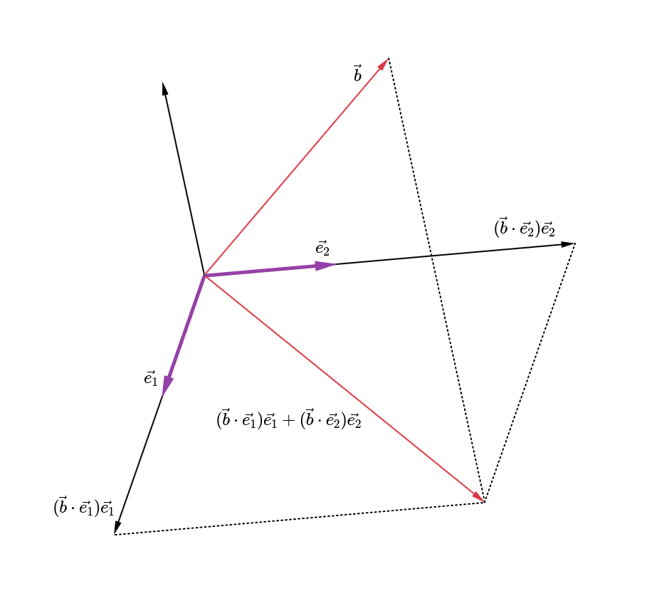
Here, the coefficient of this projection vector is called Fourier coefficient. Moreover, for a matrix $A \in \mathbb{R^{m \times n}}$ whose column vectors are a basis of a vector space $W$, the projection of $\vec{b}$ on $W$ $$\begin{aligned} Proj_{W} \vec{b} &= A \vec{b} = A(A^t A)^{-1} (A^t \vec{b}) \\ &= (\vec{b} \cdot \vec{e_1})\vec{e_1} + \cdots + (\vec{b} \cdot \vec{e_n})\vec{e_n} \end{aligned}$$

where $\{ \vec{e_1}, \cdots, \vec{e_n} \}$ is an orthogonal basis of $W$. Note that $A(A^t A)^{-1} A^t$ is the standard matrix of this orthogonal projection. Let this standard matrix be $P$. Then, $P^t = P$ which means $P$ is symmetric. Also, $P^2 = P$ which means the projected point keeps the same place after projecting again as mentioned in this note. For example, for a vector $\vec{b} \in \mathbb{R^{3 \times 1}}$, its projection on the plane $W$ is as below figure.

11. Cross Product

Other than the basic features, there are things to remember.

• Triple product $\vec{a} \cdot (\vec{b} \times \vec{c}) = \vec{b} \cdot (\vec{c} \times \vec{a}) = \vec{c} \cdot (\vec{a} \times \vec{b})$ means that the volume of the parallelepiped defined by the three vectors. So, the volume of the tetrahedron is $\vert \vec{a} \cdot (\vec{b} \times \vec{c}) \vert / 6$.
• $\vec{a} \times (\vec{b} \times \vec{c}) = (\vec{a} \cdot \vec{c})\vec{b} - (\vec{a} \cdot \vec{b})\vec{c} \ne (\vec{a} \times \vec{b}) \times \vec{c}$, so it is not associative.
• By Lagrange’s identity, $(\vec{a} \times \vec{b}) \cdot (\vec{c} \times \vec{d}) = (\vec{a} \cdot \vec{c})(\vec{b} \cdot \vec{d}) - (\vec{a} \cdot \vec{d})(\vec{b} \cdot \vec{c})$.
• Interestingly, $\Vert \vec{a} \times \vec{b} \Vert^2 + (\vec{a} \cdot \vec{b})^2 = \Vert \vec{a} \Vert^2 \Vert \vec{b} \Vert^2$.

12. Cayley-Hamilton Theorem

For a matrix $A \in \mathbb{R^{n \times n}}$ and the identity matrix $I$ of size $n$, let $D(\lambda) = \vert A - \lambda I \vert$. By observation, $D(A) = 0$. In other words, $A$ is a root of the characteristic equation $f(\lambda) = \vert A - \lambda I \vert = 0$. Here, $f(A) = 0$ is called the Cayley-Hamilton theorem. This theorem leads to the inverse matrix of $A$ as follows. Define the characteristic equation $f(\lambda) = \lambda^n + a_{n-1}\lambda^{n-1} + \cdots + a_1 \lambda + a_0 I = 0$. Then, $$\begin{aligned} f(A) &= A^n + a_{n-1}A^{n-1} + \cdots + a_1 A + a_0 I = 0 \\ \implies A^{-1} f(A) &= A^{n-1} + a_{n-1}A^{n-2} + \cdots + a_1 I + a_0 A^{-1} = 0 \\ \implies A^{-1} &= \frac{1}{a_0} \left( -A^{n-1} - a_{n-1} A^{n-2} - \cdots - a_1 I \right) \end{aligned}$$

13. Transformations

• Finding a symmetric point about a line $y = (\tan \theta)x$

$$\begin{aligned} \left(\begin{array}{cc} \cos 2 \theta & \sin 2 \theta \\ \sin 2 \theta & -\cos 2 \theta \end{array}\right) \end{aligned}$$

• Finding a projected point about a line $y = (\tan \theta)x$

$$\begin{aligned} \left(\begin{array}{cc} \cos^2 \theta & \sin \theta \cos \theta \\ \sin \theta \cos \theta & \sin^2 \theta \end{array}\right) \end{aligned}$$

• Finding a symmetric point about a plane $n \cdot x = 0$ where $n$ is the normal

$$\begin{aligned} I - 2 \cfrac{n n^t}{n^t n} \end{aligned}$$

• Finding a projected point about a plane $n \cdot x = 0$ where $n$ is the normal

$$\begin{aligned} I - \cfrac{n n^t}{n^t n} \end{aligned}$$

14. Jacobian

As if the substitution method in a definite integral causes the size of variables to change such as $x^2 = t \to 2xdx = dt$, the substitution method in a double integral makes the region area change. Therefore, this difference must be compensated, which is what the Jacobian determinant does. Meanwhile, geometrically the Jacobian determinant also means the instantaneous rate of change of area. Suppose $f: \mathbb{R}^n \to \mathbb{R}^m$ is a function such that each of its first-order partial derivatives exists on $\mathbb{R}^n$. This function takes a point $x \in \mathbb{R}^n$ as input and produces the vector $f(x) \in \mathbb{R}^m$ as output. Then the Jacobian matrix $J \in \mathbb{R}^{m \times n}$ is defined as follows. $$\begin{aligned} J = \left(\begin{array}{c} \nabla^t f_1 \\ \vdots \\ \nabla^t f_m \end{array}\right) = \left(\begin{array}{ccc} \cfrac{\partial f_1}{\partial x_1} & \cdots & \cfrac{\partial f_1}{\partial x_n} \\ \vdots & \ddots & \vdots \\ \cfrac{\partial f_m}{\partial x_1} & \cdots & \cfrac{\partial f_m}{\partial x_n} \end{array}\right) \end{aligned}$$

where $\nabla^t f_i$ is the transpose of the gradient of the $i$-th component. Now, assume that $x = f(u, v)$ and $y = g(u, v)$. Then, the Jacobian determinant is $$\begin{aligned} \vert J \vert = \left \vert \cfrac{\partial (x, y)}{\partial (u, v)} \right \vert = \left \vert \begin{array}{cc} x_u & x_v \\ y_u & y_v \end{array} \right \vert = \cfrac{1}{\left \vert \cfrac{\partial (u, v)}{\partial (x, y)} \right \vert} = \cfrac{1}{ \left \vert \begin{array}{cc} u_x & u_y \\ v_x & v_y \end{array} \right \vert } \end{aligned}$$

Moreover, if $\vert J \vert = 0$, there exists a functional relationship between $x$ and $y$. As such, the transformation is not invertible, which means that there is no way to get $x$ and $y$ back from $u$ and $v$. Similarly, assume that $x = f(u, v, t)$, $y = g(u, v, t)$, and $z = h(u, v, t)$. Then, the Jacobian determinant is $$\begin{aligned} \vert J \vert = \left \vert \cfrac{\partial (x, y, z)}{\partial (u, v, t)} \right \vert = \left \vert \begin{array}{ccc} x_u & x_v & x_t \\ y_u & y_v & y_t \\ z_u & z_v & z_t \end{array} \right \vert \end{aligned}$$

Again, if $\vert J \vert = 0$, there exists a functional relationship between $x$, $y$, $z$. As such, the transformation is not invertible, which means that there is no way to get $x$, $y$, $z$ back from $u$, $v$, $t$.