Normal Equation

• The Residual Minimization
• Another Approach When $m > n$
• Another Approach Using Projector
• Evaluation
• Reference

For an $m \times n$ matrix $A$ and a vector $b \in \mathbb{R}^m$, the linear system $Ax = b$ is to find the optimal solution $x \in \mathbb{R}^n$.

The Residual Minimization

The problem $Ax = b$ can be replaced by the problem minimizing the residual, $\left\| b - Ax \right\|_2^2$. Let $A_i$ be the $i$-th row vector of $A$. Then the cost function $f(x)$ can be defined as follows. $$\begin{aligned} f(x) &= \left\| b - Ax \right\|_2^2 = \left\| \left(\begin{array}{c} b_1 - A^t_1 x \\ \vdots \\ b_m - A^t_m x \end{array}\right) \right\|_2^2 = \sum_{k} (b_k - A^t_k x)^2 \end{aligned}$$

A necessary condition for a minimum is that $x$ be a critical point of $f$, where the gradient vector $\nabla f(x)$ is zero. Let $a_{ij}$ be the $(i, j)$ element of $A$. Then, $$\begin{aligned} \frac{\partial f}{\partial x_i} &= \sum_{k} 2(b_k - A^t_k x) \frac{\partial}{\partial x_i} (b_k - A^t_k x) = 2 \sum_{k} (b_k - A^t_k x) (- a_{ki}) = 0 \\ &\implies \sum_{k} a_{ki} A^t_k x = \sum_{k} a_{ki} b_k = \left(\begin{array}{ccc} a_{1i} & \cdots & a_{mi} \end{array}\right) \left(\begin{array}{c} A^t_1 \\ \vdots \\ A^t_m \end{array}\right) x = \left(\begin{array}{ccc} a_{1i} & \cdots & a_{mi} \end{array}\right) \left(\begin{array}{c} b_1 \\ \vdots \\ b_m \end{array}\right) \\ &\implies \left(\begin{array}{ccc} a_{11} & \cdots & a_{m1} \\ & \vdots & \\ a_{1n} & \cdots & a_{mn} \end{array}\right) \left(\begin{array}{c} A^t_1 \\ \vdots \\ A^t_m \end{array}\right) x = \left(\begin{array}{ccc} a_{11} & \cdots & a_{m1} \\ & \vdots & \\ a_{1n} & \cdots & a_{mn} \end{array}\right) \left(\begin{array}{c} b_1 \\ \vdots \\ b_m \end{array}\right) \\ \\ &\implies \color{red}{A^tAx = A^t b} \end{aligned}$$

This equation is called normal equation. Moreover, $A^tA$ is positive (semi-)definite because $x^t A^t Ax = (Ax)^t (Ax) = \left\| Ax \right\|_2^2 \ge 0$, so it minimizes $f$. Especially, if $\left\| Ax \right\|_2^2 \not = 0$, it tells that there is no $x$ such that $Ax = \mathbf{0}$ except $x = \mathbf{0}$. It also means that $A$ is nonsingular whose column vectors are linearly independent. Therefore, the solution of $A^t Ax = A^t b$ is the same as the optimal solution of $Ax = b$ when $A$ is nonsingular.

Another Approach When $m > n$

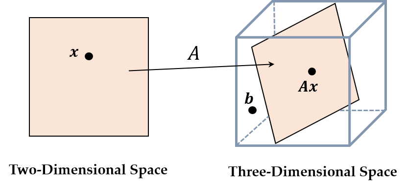
In this case, $A$ maps the lower dimension to the higher dimension. For example, when $m = 3$ and $n = 2$, there may be a point $b$ in the objective space that $Ax$ cannot completely cover.

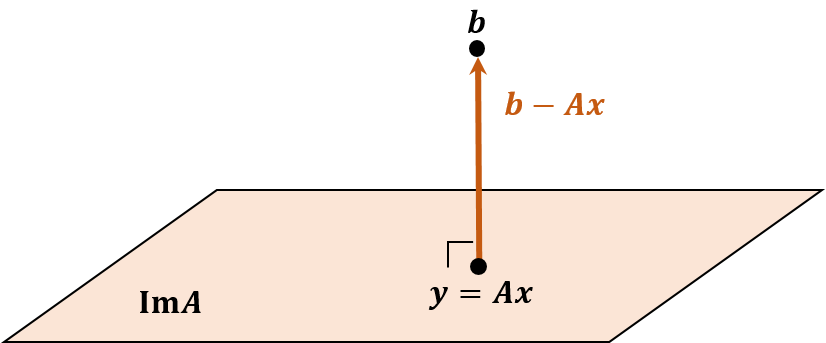
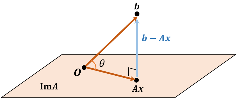
So, the linear system $Ax = b$ cannot be solved exactly. However, finding the point closest to $b$ might be a good approximation. Let $y = Ax$ be the closest point to $b$.

When $y$ is closest to $b$, the vector $b - y = b - Ax$ is parallel to the normal of the hyperplane $Im A$. Besides, $Ae_1, \cdots, Ae_n$ are the basis of $Im A$ where $e_1, \cdots, e_n$ are the standard basis of the original space. In other words, it implies that column vectors of $A$ are the basis of $Im A$, which means they are all perpendicular to $b - Ax$. Therefore, $A^t (b - Ax) = \mathbf{0}$, and it yields the normal equation. Accordingly, the normal equation estimates the optimal solution of $Ax = b$ even though there exists no the exact solution.

Another Approach Using Projector

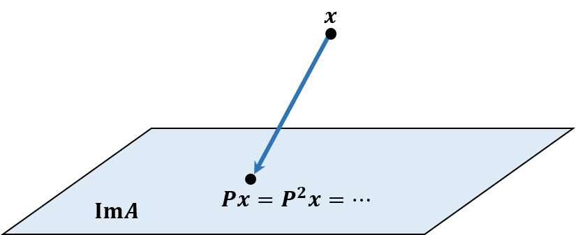
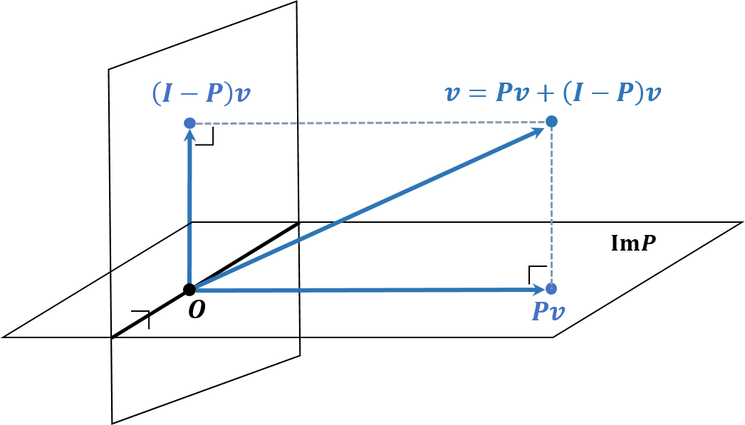
A square matrix $P$ is called a projector if it is idempotent, which means $P^2 = P$. Such $P$ projects any vector to $Im P$ but leaves unchanged any vector that is already on $Im P$. If $P$ is symmetric, it is called an orthogonal projector, and $I - P$ is also an orthogonal projector to a hyperplane perpendicular to $Im P$. Obviously, $(I - P)^2 = I - 2P + P^2 = I - P$. More specifically, for any vector $v = Pv + (I - P)v$, $$\begin{aligned} (Pv)^t ((I - P)v) &= v^t P^t (v - Pv) = v^t P (v - Pv) \\ &= v^t P v - v^t P^2 v = v^t P v - v^t P v = 0 \\ \\ \implies &Pv \perp (I - P)v \end{aligned}$$

Now, assume that $P$ is an orthogonal projector onto $\text{span}(A)$ such that $PA = A$. Then the cost function $f(x)$ can be derived as follows. $$\begin{aligned} f(x) = \left\| b - Ax \right\|^2_2 &= \left\| P(b - Ax) + (I - P)(b - Ax) \right\|^2_2 \\ &= \left\| P(b - Ax) \right\|^2_2 + \left\| (I - P)(b - Ax) \right\|^2_2 \\ &= \left\| Pb - PAx \right\|^2_2 + \left\| (I - P)b - (I - P)Ax \right\|^2_2 \\ &= \left\| Pb - Ax \right\|^2_2 + \left\| (I - P)b \right\|^2_2 \end{aligned}$$

Note that $(I - P)A = \mathbf{0}$ since $PA = A$. The second term does not depend on $x$, so the residual norm is minimized when $x$ is chosen so that the first term is zero. $$\begin{aligned} Pb - Ax = \mathbf{0} \implies A^t(Pb - Ax) &= A^t Pb - A^t Ax = A^t P^t b - A^t Ax \\ &= (PA)^t b - A^t Ax = A^t b - A^t Ax = \mathbf{0} \end{aligned}$$

Therefore, it produces the normal equation as well.

Evaluation

The solution from the normal equation can be evaluated by the condition number and angle between $b$ and $Ax$. The condition number of $A$ tells how close $A$ is a singular matrix. However, if $m \not = n$, $A$ is not invertible, so the pseudoinverse $A^{+} = (A^t A)^{-1} A^t$ should be introduced. In this case, the condition number of $A$ is $$\begin{aligned} Cond_2 (A) = \left\| A \right\|_2 \left\| A^{+} \right\|_2 \end{aligned}$$

Meanwhile, as the angle between $b$ and $Ax$ is smaller, $b$ is closer to $Ax$, so it is a good measure to find whether the solution is well-conditioned. This angle can be obtained as $\cos \theta = \left\| Ax \right\|_2 / \left\| b \right\|_2$.

Reference

[1] Michael T. Heath, Scientific Computing: An Introductory Survey. 2nd Edition, McGraw-Hill Higher Education.