Conjugate Gradient Method

• Minimization
• Eigenvectors & Eigenvalues
• Conjugate Gradient Method
• Gram-Schmidt Conjugation
• Only New Search Direction
• Preconditioning
• Normal Equation
• Nonlinear Conjugate Gradient Method
• References

Minimization

The conjugate gradient method is the most popular iterative method for solving large systems of linear equations. This is effective for systems of the form $Ax=b$ where $x$ is an unkown vector, $b$ is a known vector, and $A$ is a known, square, symmetric, positive-definite matrix. This form is mostly used to find the minimum of a cost function $f(x)$. Since $A$ is a symmetric and positive-definite matrix, $f(x)$ is shaped like a paraboloid bowl, so it has a minimum as mentioned in this note. If $A$ might be singular, in which case no solution is unique. In this case, the set of solutions is a line or hyperplane having a uniform value for $f$. If $A$ is indefinite, the gradient descent and conjugate gradient methods will likely fail.

Eigenvectors & Eigenvalues

Consider an eigenvector $v$ and an eigenvalue $\lambda$ of a matrix $B$ such that $Bv = \lambda v$. Iterative methods often depend on applying $B$ to a vector over and over again. When $B$ is repeatedly applied to an eigenvector $v$, one of two things can happen. If $\vert \lambda \vert < 1$, then $B^iv = \lambda^iv$ will vanish as $i$ approaches infinity. If $\vert \lambda \vert > 1$, then $B^iv$ will grow to infinity. Each time $B$ is applied, the vector grows or shrinks according to the value of $\vert \lambda \vert$.

If $B$ is symmetric, then all different eigenvectors of $B$ are perpendicular. That is, all eigenvectors form a basis for $\mathbb{R}^n$. As such, any $n$-dimensional vector can be expressed as a linear combination of these eigenvectors. Applying $B$ to $x$ that is not an eigenvector is equivalent to applying $B$ to the eigenvectors and summing the result.

Conjugate Gradient Method

The conjugate gradient method is especially suitable for very large problems since it does not require explicit second derivatives. Indeed, it does not even store an approximation to the Hessian matrix. While the gradient descent method tends to search in the same directions repeatedly, leading to very slow convergence, the conjugate gradient method avoids repeatedly searching the same directions by modifying the new gradient at each step to remove components in previous directions. The resulting sequence of conjugate search directions implicitly accumulates information about the Hessian matrix as iterations proceed. Compare that the gradient descent method follows a zigzag path, which appears because each gradient is orthogonal to the previous gradient.

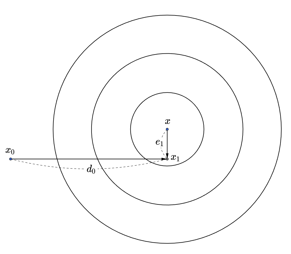
Here is the idea behind this method. Suppose that $d_0, d_1, \cdots, d_{n-1}$ are a set of orthogonal search directions whose each search direction is used for exactly one step. Let $x_1, \cdots, x_n$ be the estimated solutions by step starting from the initial guess $x_0$. Also, let the error in $i$-step be $e_i = x_i - x$ to indicate how far from the solution $x$. Then, $e_{i+1}$ should be orthogonal to $d_i$ so that $d_i$ will never be used again. Using this fact, $x_i$ can be updated along with $\alpha_i$ per one-iteration where $\alpha_i$ is a line search parameter that indicates how big a step takes. $$\begin{aligned} &x_{i+1} = x_i + \alpha_i d_i \\\\ \implies &d_i^t e_{i+1} = d_i^t (x_{i+1} - x) = d_i^t (x_i + \alpha_i d_i - x) = d_i^t (e_i + \alpha_i d_i) = 0 \\ \implies &\alpha_i = -\cfrac{d_i^t e_i}{d_i^t d_i} \end{aligned}$$

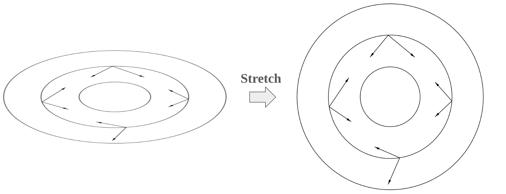
However, the contradiction occurs $\alpha_i$ requires $e_i$ to update $x_i$ and $e_i$ needs the solution $x$. The workaround is to make the search directions mutually $A$-orthogonal. Vectors $y$ and $z$ are called $A$-orthogonal if $y^t Az = 0$, or conjugate. That is, $y$ is orthogonal to the transformed $z$ by $A$. As shown below, the main idea is to stretch the ellipses to appear circular. In this perspective, $e_{i+1}$ should be $A$-orthogonal to $d_i$ this time.

Considering that the residual $r_i = b - Ax_i = Ax - Ax_i = -Ae_i$ which indicates how far from the correct value of $b$, $$\begin{aligned} d_i^t A e_{i+1} &= d_i^t A (x_{i+1} - x) = d_i^t A(x_i + \alpha_i d_i - x) = d_i^t A(e_i + \alpha_i d_i) \\ &= d_i^t A e_i + \alpha_i d_i^t A d_i = -d_i^t r_i + \alpha_i d_i^t A d_i = 0 \\ &\implies \alpha_i = \cfrac{d_i^t r_i}{d_i^t A d_i} \end{aligned}$$

Gram-Schmidt Conjugation

Then how can the search directions be obtained? The conjugate Gram-Schmidt process makes it simple to generate them. Recalling the Gram-Schmidt process, it is a method of constructing an orthonormal basis from a linearly independent set of vectors. More specifically, $d_i$ can be constructed from a set of $n$ linearly independent vectors $u_0, \cdots, u_{n-1}$ as follows. $$\begin{aligned} d_0 &= u_0, \\ d_1 &= u_1 - (u_1 \cdot d_0)d_0, \\ d_2 &= u_2 - (u_2 \cdot d_0)d_0 - (u_2 \cdot d_1)d_1, \\ &\vdots \\ d_i &= u_i - \sum_{k=0}^{i-1} (u_i \cdot d_k)d_k \end{aligned}$$

Note that these should be normalized later. But, how is this formula derived? This is based on the orthogonality. $$\begin{aligned} &d_i = u_i + \sum_{k=0}^{i-1} \beta_{ik} d_k \\ \implies &0 = d_i \cdot d_j = u_i \cdot d_j + \sum_{k=0}^{i-1} \beta_{ik} (d_k \cdot d_j) = u_i \cdot d_j + \beta_{ij} (d_j \cdot d_j) = u_i \cdot d_j + \beta_{ij} \quad (i > j)\\ \implies &\beta_{ij} = -u_i \cdot d_j \end{aligned}$$

The same logic is used for the conjugate Gram-Schmidt process. This is based on the $A$-orthogonality this time. $$\begin{aligned} &d_i = u_i + \sum_{k=0}^{i-1} \beta_{ik} d_k \\ \implies &0 = d_i^t A d_j = u_i^t A d_j + \sum_{k=0}^{i-1} \beta_{ik} d_k^t A d_j = u_i^t A d_j + \beta_{ij} d_j^t A d_j \quad (i > j)\\ \implies &\beta_{ij} = -\cfrac{u_i^t A d_j}{d_j^t A d_j} \end{aligned}$$

Then how can the set $\{ u_0, \cdots, u_{n-1} \}$ selected? It is possible by setting $u_i = r_i$, that is, by conjugation of the residuals. This choice makes sense because the residual has the nice property that it is orthogonal to the previous search directions. In other words, it is guaranteed always to produce a new, linearly independent search direction unless the residual is zero, in which case the problem is already solved. $$\begin{aligned} d_j^t r_i &= -d_j^t Ae_i = -d_j^t A(x_i - x) = -d_j^t A(x_{i-1} + \alpha_{i-1} d_{i-1} - x) \\ &= -d_j^t A(e_{i-1} + \alpha_{i-1} d_{i-1}) = d_j^t r_{i-1} - \alpha_{i-1} d_j^t A d_{i-1} \\ &= \cdots = d_j^t r_{j} - \sum_{k=j}^{i-1} \alpha_{k} d_j^t A d_{k} = d_j^t r_{j} - \alpha_{j} d_j^t A d_{j} = d_j^t r_{j} - d_j^t r_{j} = 0 \quad (i > j) \end{aligned}$$

Note that the residual has the recurrence property. As each residual is orthogonal to the previous search directions, it is also orthogonal to the previous residuals. That is, $r_i^t r_j = 0$ when $i \ne j$. $$\begin{aligned} d_j = u_j + \sum_{k=0}^{j-1} \beta_{jk} d_k \implies 0 = d_j^t r_i = u_j^t r_i + \sum_{k=0}^{j-1} \beta_{jk} d_k^t r_i = u_j^t r_i = r_j^t r_i \quad (i > j, u_j = r_j) \end{aligned}$$

As another important property, the following identity updates $\alpha_i$. $$\begin{aligned} d_i^t r_i = u_i^t r_i + \sum_{k=0}^{i-1} \beta_{ik} d_k^t r_i = u_i^t r_i = r_i^t r_i \implies \alpha_i = \cfrac{d_i^t r_i}{d_i^t A d_i} = \cfrac{r_i^t r_i}{d_i^t A d_i} \end{aligned}$$

Only New Search Direction

Since the search directions can be obtained from the conjugate Gram-Schmidt process, the final update function can be set up as well. From the recurrence of the residual checked previously, $r_{j+1} = r_j - \alpha_j A d_j$, $$\begin{aligned} r_i^t r_{j+1} &= r_i^t r_j - \alpha_j r_i^t A d_j \implies \alpha_j r_i^t A d_j = r_i^t r_j - r_i^t r_{j+1} \\\\ r_i^t A d_j &= \begin{cases} \; \cfrac{r_i^t r_i}{\alpha_i} & (i = j) \\ \; -\cfrac{r_i^t r_i}{\alpha_{i-1}} & (i = j + 1) \\ \; 0 & \text{otherwise} \end{cases} \\\\ \beta_{ij} &= -\cfrac{u_i^t A d_j}{d_j^t A d_j} = -\cfrac{r_i^t A d_j}{d_j^t A d_j} = \begin{cases} \; \cfrac{1}{\alpha_{i-1}} \cfrac{r_i^t r_i}{d_{i-1}^t A d_{i-1}} & (i = j + 1) \\ \; 0 & (i > j + 1) \end{cases} \end{aligned}$$

Note that $\beta_{ij}$ is defined only when $i > j$. This result shows that most of the $\beta_{ij}$ terms have disappeared. It is no longer necessary to store old search directions to ensure the $A$-orthogonality of new search directions. This major property reduces the space and time complexities per iteration to $O(m)$, where $m$ is the number of nonzero entries of $A$. Simplyfing $\beta_{i, i-1}$ further, $$\begin{aligned} \alpha_i = \cfrac{r_i^t r_i}{d_i^t A d_i} \implies \beta_{i, i-1} = \cfrac{1}{\alpha_{i-1}} \cfrac{r_i^t r_i}{d_{i-1}^t A d_{i-1}} = \cfrac{r_i^t r_i}{r_{i-1}^t r_{i-1}} \end{aligned}$$

As a result, the conjugate gradient method can be summed up as follows. $$\begin{aligned} \begin{cases} \; d_0 = r_0 = b - A x_0 \\ \; \alpha_i = \cfrac{r_i^t r_i}{d_i^t A d_i} \\ \; x_{i+1} = x_i + \alpha_i d_i \\ \; r_{i+1} = r_i - \alpha_i A d_i \\ \; \beta_{i+1, i} = \cfrac{r_{i+1}^t r_{i+1}}{r_{i}^t r_{i}} \\ \; d_{i+1} = r_{i+1} + \beta_{i+1} d_i \end{cases} \end{aligned}$$

Then how to choose a starting point, and when to stop? If a rough estimate of the value of $x$ is available, it can be used as the starting point $x_0$. If not, set $x_0 = \mathbf{0}$. This will eventually converge when used to solve linear systems. Nonlinear minimization is trickier, though, because there may be several local minima. Usually, it is customary to stop when the norm of the residual falls below a specific value such as $\Vert r_i \Vert < \epsilon \Vert r_0 \Vert$.

Preconditioning

Thd conjugate gradientn method can still converge very slowly if $A$ is ill-conditioned. Preconditioning is a technique for improving the condition number of a matrix. Suppose that $M$ is a symmetric, positive-definite matrix that approximates $A$, but is easier to invert. Then, $Ax=b$ can be indirectly solved by solving $M^{-1}Ax = M^{-1}b$ because $M^{-1}A$ is relatively well-conditioned. If the eigenvalues of $M^{-1}A$ are better clustered than those of $A$, this system can be iteratively solved more quickly than the original problem. But, $M^{-1}A$ is not generally symmetric nor definite, even if $M$ and $A$ are. To avoid this difficulty, $E$ can be obtained such that $EE^t = M$ by Cholesky factorization since $M$ is positive-definite. Then, $M^{-1}A$ and $E^{-1}AE^{-t}$ have the same eigenvalues. Let $v$ be an eigenvector of $M^{-1}A$ with eigenvalue $\lambda$. $$\begin{aligned} (E^{-1}AE^{-t})(E^t v) = E^{-1} Av = (E^t E^{-t})E^{-1} Av = E^t M^{-1} Av = \lambda E^t v \end{aligned}$$

With this fact, the system $Ax=b$ can be transformed into $$\begin{aligned} Ax = b \implies E^{-1}Ax = E^{-1}b \implies (E^{-1}AE^{-t})E^t x = E^{-1}b \implies (E^{-1}AE^{-t})\hat{x} = E^{-1}b \end{aligned}$$

So, $x$ can be obtained after solving it for $\hat{x} = E^t x$ first. Note that $E^{-1}AE^{-t}$ is symmetric and positive-definite. Then, the transformed preconditioned conjugate gradient method as follows. $$\begin{aligned} \hat{A} = E^{-1}AE^{-t}, \quad \hat{b} &= E^{-1}b, \quad \hat{x} = E^t x \\\\ \hat{r}_0 = E^{-1}b - (E^{-1}AE^{-t})E^t x_0 &= E^{-1}(b - Ax_0) \implies \hat{r}_0 = E^{-1}r_0 \\\\ \hat{d}_{i}^t \hat{A} \hat{d}_j = \hat{d}_{i}^t E^{-1}AE^{-t} \hat{d}_j = 0 &\implies d_i = E^{-t} \hat{d}_i \implies \hat{d}_i = E^t d_i \end{aligned}$$

The difficulty is that $E$ must be computed. However, there is a way to avoid this computation. Considering that $\hat{r}_i^t \hat{r}_i = r_i^t E^{-t}E^{-1} r_i = r_i^t M^{-1} r_i$ since $E^{-t}E^{-1} = M^{-1}$, the untransformed preconditioned conjugate gradient method is finally updated as follows. $$\begin{aligned} \begin{cases} \; r_0 = b - A x_0 \\\\ \; \hat{d}_0 = \hat{r}_0 \implies d_0 = E^{-t}E^{-1} r_0 = M^{-1} r_0 \\\\ \; \alpha_i = \cfrac{\hat{r}_i^t \hat{r}_i}{\hat{d}_i^t \hat{A} \hat{d}_i} = \cfrac{r_i^t M^{-1} r_i}{d_i^t E E^{-1} A E^{-t} E^t d_i} = \cfrac{r_i^t M^{-1} r_i}{d_i^t A d_i} \\\\ \; x_{i+1} = x_i + \alpha_i d_i \\\\ \; r_{i+1} = r_i - \alpha_i A d_i \\\\ \; \beta_{i+1, i} = \cfrac{\hat{r}_{i+1}^t \hat{r}_{i+1}}{\hat{r}_{i}^t \hat{r}_{i}} = \cfrac{r_{i+1}^t M^{-1} r_{i+1}}{r_{i}^t M^{-1} r_{i}} \\\\ \; d_{i+1} = M^{-1} r_{i+1} + \beta_{i+1} d_i \end{cases} \end{aligned}$$

As shown above, $E$ disappear and only $M^{-1}$ is required. The effectiveness of a preconditioner $M$ is determined by the condition number of $M^{-1}A$, and occasionally by its clustering of eigenvalues. The problem remains of finding a preconditioner that approximates $A$ well enough to improve convergence enough to make up for the cost of computing $M^{-1}r_i$ once per iteration. Intuitively, preconditioning is an attempt to stretch the quadratic form to make it appear more spherical so that the eigenvalues are close to each other. A perfect preconditioner is $M=A$ which makes $M^{-1}r_i$ have a condition number of one, and the quadratic form is perfectly spherical, so the solution takes only one iteration.

The simplest preconditioner is a diagonal matrix whose diagonal entries are identical to those of $A$, known as diagoanl preconditioning or Jacobi preconditioning, which is scaling the quadratic form along the coordinate axes. By comparison, the perfect preconditioner $M=A$ scales the quadratic form along its eigenvector axes.

A more elaborate preconditioner is incomplete Cholesky preconditioning. While the Cholesky factorization finds $L$ such that $A=LL^t$, incomplete Cholesky factorization finds $\hat{L}$ such that $A \approx \hat{L}\hat{L}^t$ where $\hat{L}$ might be restricted to have the same pattern of nonzero elements as $A$ and other elements of $L$ are thrown away. To use $\hat{L}\hat{L}^t$ as a preconditioner, the solution to $\hat{L}\hat{L}^t w = z$ is computed by backsubstitution. Unfortunately, incomplete Cholesky preconditioning is not always stable.

Normal Equation

What if $A$ is not square, not symmetric, and not positive-definite? In this case, the normal equation should be applied, which means that the solution can be found from the linear system $A^tAx = A^tb$. If $A$ is square and nonsingular, the solution is the same as the one of $Ax=b$. If $A$ is not square, and $Ax=b$ is overconstrained, then there may or may not be a solution to $Ax=b$, but it is always possible to find $x$ closest to the solution. If $Ax=b$ is not underconstrained, then $A^t A$ is nonsingular since $A^t A$ is symmetric and positive-definite, and the conjugate gradient method can be used to solve this normal equation. However, note that the condition number of $A^t A$ is the square of that of $A$, so convergence is significantly slower.

Nonlinear Conjugate Gradient Method

As explained in this note, suppose that $f$ is a function for $x \in \mathbb{R}^n$ and its Hessian matrix $H_f$ is positive definite. By Taylor’s theorem, $$\begin{aligned} f(x + s) \approx f(x) + \nabla f(x)^t s + \frac{1}{2} s^t H_f(x) s \end{aligned}$$

That is, $x$ should be moved by $\Vert s \Vert$ in direction $s$. However, the direction to move in the case of the conjugate gradient method is already fixed as $d$. As such, what to know is how much $x$ should be moving by. More specifically, $\alpha$ such that $s = \alpha d$ should be selected. To find $\alpha$, the approximated equation should be differentiated against $\alpha$, not $s$ this time, unlike the original process mentioned in this note. $$\begin{aligned} \alpha d^t H_f(x) d = - \nabla f(x)^t d \end{aligned}$$

References

[1] An Introduction to the Conjugate Gradient Method Without the Agonizing Pain

[2] Michael T. Heath, Scientific Computing: An Introductory Survey. 2nd Edition, McGraw-Hill Higher Education.