Variance Shadow Maps

• 1. Percentage-Closer Filtering(PCF)
• 2. Variance Shadow Map(VSM)
• 3. Parallel-Split Variance Shadow Map(PSVSM)
• 4. Summed Area Table Variance Shadow Map(SATVSM)
  • Light Bleeding
• References
• Code

The shadow map algorithm is to create shadow using the depth image from a light view. Similarly, the variance shadow map uses variance of depths to reduce antialiasing. Along with introducing this, several algorithms are tested together for comparison.

1. Percentage-Closer Filtering(PCF)

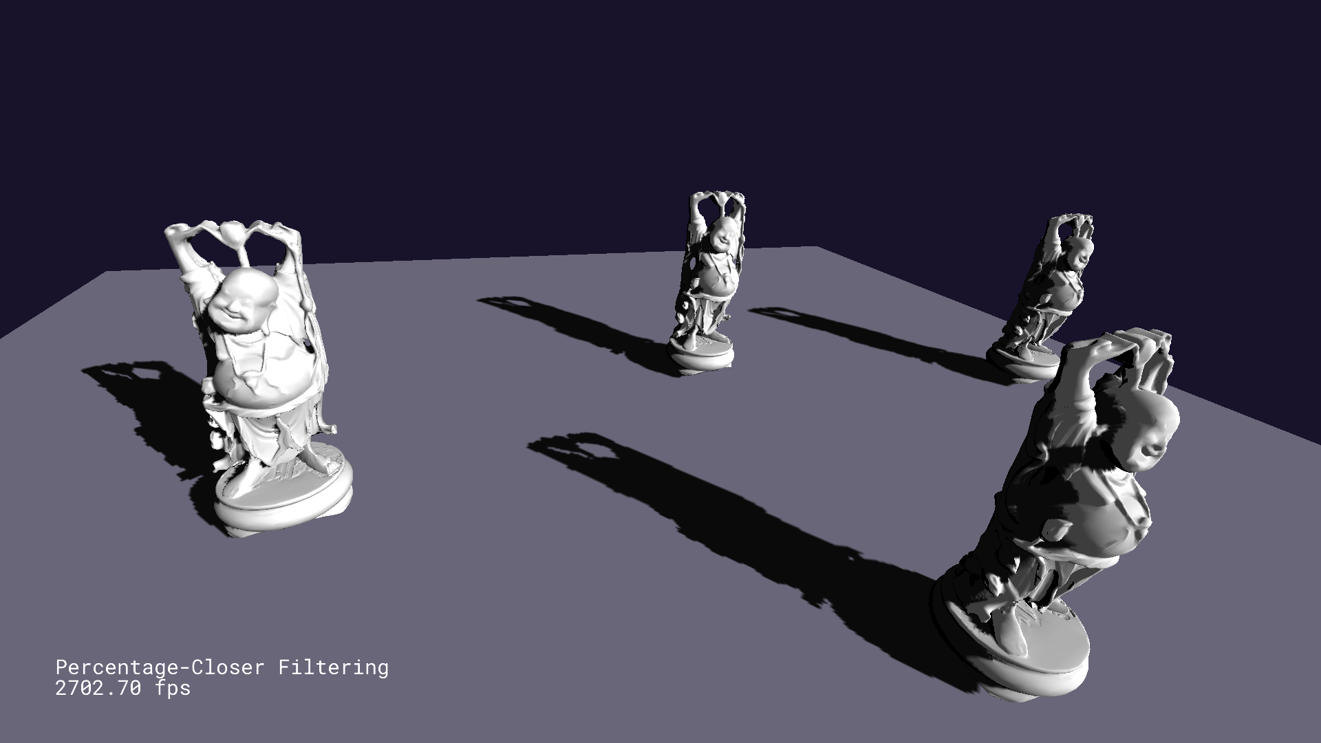
To resolve the antialiasing problem, PCF averages depths to reference[1]. It is acting like a box blur algorithm, which means it costs by a filter size. Therefore, the filter size can be selected adaptively, and [2] suggests to use derivatives of depth map texture coordinates. In short, the filter size gets decreased when the camera is closer, and increased when the camera is farther. Besides this handling, the depth value should be biased since PCF suffers the shadow acne problem.

2. Variance Shadow Map(VSM)

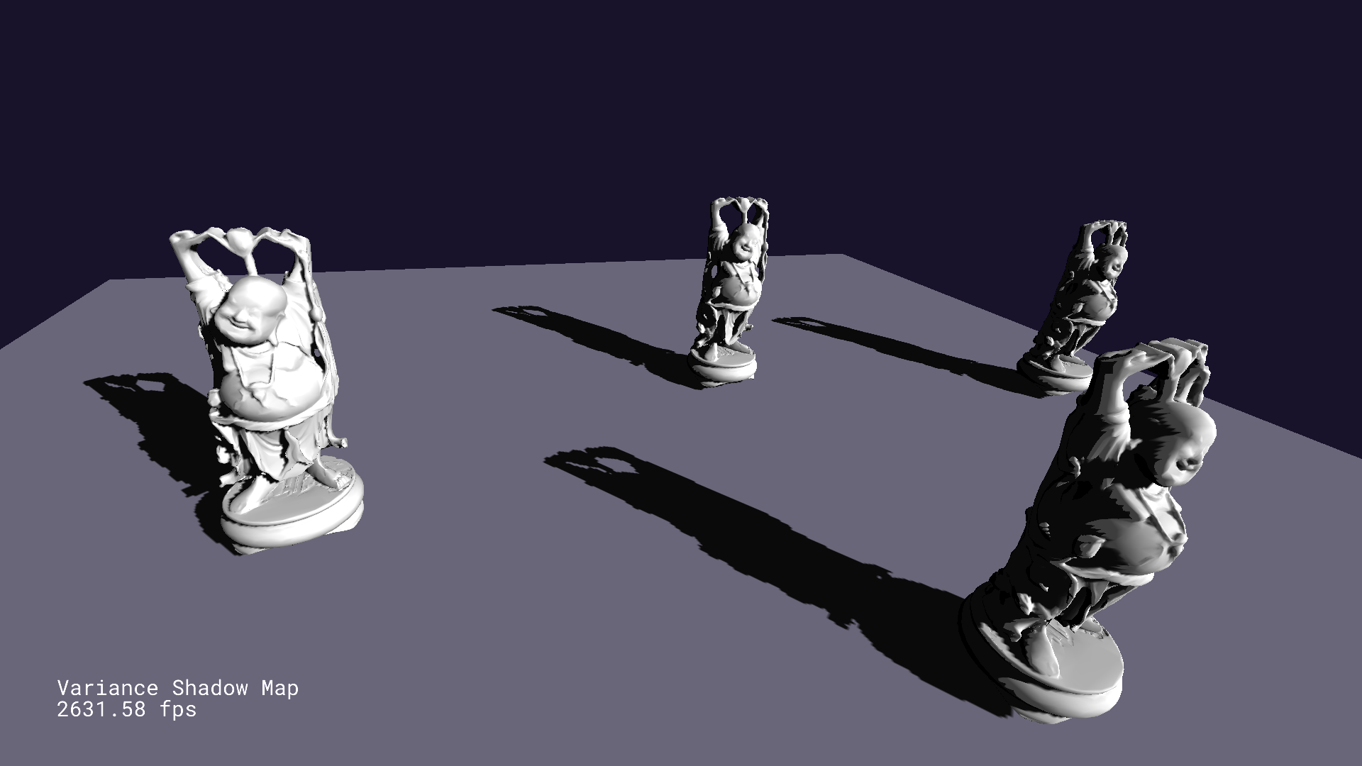
VSM is working similarly with standard shadow maps, but it stores depth $M_1$ and depth squared $M_2$ called moments for the light view texture. The key point is to assmume that the current depth value represents the expectation of depths. $$\begin{aligned} M_1 &= E[x] = \int xp(x) dx \\ M_2 &= E[x^2] = \int x^2 p(x) dx \end{aligned}$$

With this moments, the mean $\mu = M_1$ and variance $\sigma^2 = M_2 - M_1^2$ can be derived. Given these mean and variance, an upper bound on the probability that the current surface is lit can be drawn by applying Chebyshev’s inequality. To be specific, what to compute is how likely the current depth $t$ which is the distance from the current surface to a light source is smaller, $P(X \geq t)$. For this, the one-sided Chebyshev inequality is only required, so Cantelli’s inequality is more suitable. For any $u \geq 0$, $$\begin{aligned} P(X \geq t) = P(X - \mu + u \geq t - \mu + u). \end{aligned}$$

Let $\lambda = t - \mu$ and $Y = X - \mu$, then $E[Y] = 0$ and $Var[Y] = E[(Y - E[Y])^2] = E[(X - \mu)^2] = \sigma^2$. From this fact, $$\begin{aligned} P(X \geq t) &= P(X - \mu + u \geq t - \mu + u) = P(Y + u \geq \lambda + u) \\ &\leq P(Y + u \geq \lambda + u) + P(Y + u \leq -(\lambda + u)) \\ &= P((Y + u)^2 \geq (\lambda + u)^2). \end{aligned}$$

Meanwhile, Markov’s inequality gives the following upper bound. If $X$ is a nonnegative random variable and $a > 0$, $$\begin{aligned} E[X] &= \int_{-\infty}^{\infty} xp(x) dx = \int_{0}^{\infty} xp(x) dx \\ &= \int_{0}^{a} xp(x) dx + \int_{a}^{\infty} xp(x) dx \geq \int_{a}^{\infty} xp(x) dx \\ &\geq \int_{a}^{\infty} ap(x) dx = a \int_{a}^{\infty} p(x) dx = a P(X \geq a). \end{aligned}$$

Going back to Cantelli’s inequality from this result, $$\begin{aligned} P(X \geq t) &\leq P((Y + u)^2 \geq (\lambda + u)^2) \leq \frac{E[(Y + u)^2]}{(\lambda + u)^2} \\ &= \frac{E[Y^2] + 2uE[Y] + u^2}{(\lambda + u)^2} = \frac{\sigma^2 + u^2}{(\lambda + u)^2} = g(u). \end{aligned}$$

By differentiating $g(u)$, the extremum $u_*$ can be found. $$\begin{aligned} g'(u) &= \frac{2u(\lambda + u)^2 - 2(\sigma^2 + u^2)(\lambda + u)}{(\lambda + u)^4} = \frac{2(u\lambda - \sigma^2)}{(\lambda + u)^3} = 0 \\ u_* &= \frac{\sigma^2}{\lambda} \end{aligned}$$

Consequently, Cantelli’s inequality is derived. $$\begin{aligned} P(X \geq t) &\leq g(u) \leq \frac{\sigma^2 + u_*^2}{(\lambda + u_*)^2} = \frac{\sigma^2 + \sigma^4 / \lambda^2}{(\lambda + \sigma^2 / \lambda)^2} = \frac{\lambda^2 \sigma^2 + \sigma^4}{(\lambda^2 + \sigma^2)^2} = \frac{\sigma^2 (\lambda^2 + \sigma^2)}{(\lambda^2 + \sigma^2)^2} = \frac{\sigma^2}{\lambda^2 + \sigma^2} \\ &= \frac{\sigma^2}{(t - \mu)^2 + \sigma^2} \end{aligned}$$

This inequality gives a valid upper bound only when $t \geq \mu$. If $t < \mu$, the upper bound must be $1$ because the surface is fully lit. While calculating variance, it is better to clamp the minimum variance to a small value such as $10^{-6}$ according to [2]. This clamping handles any numeric issues.

3. Parallel-Split Variance Shadow Map(PSVSM)

This algorithm is based on parallel-split shadow mapping as discussed before. However, it is combined with variance shadow maps, so it is using the upper bound from Cantelli’s inequality when calculating a shadow value.

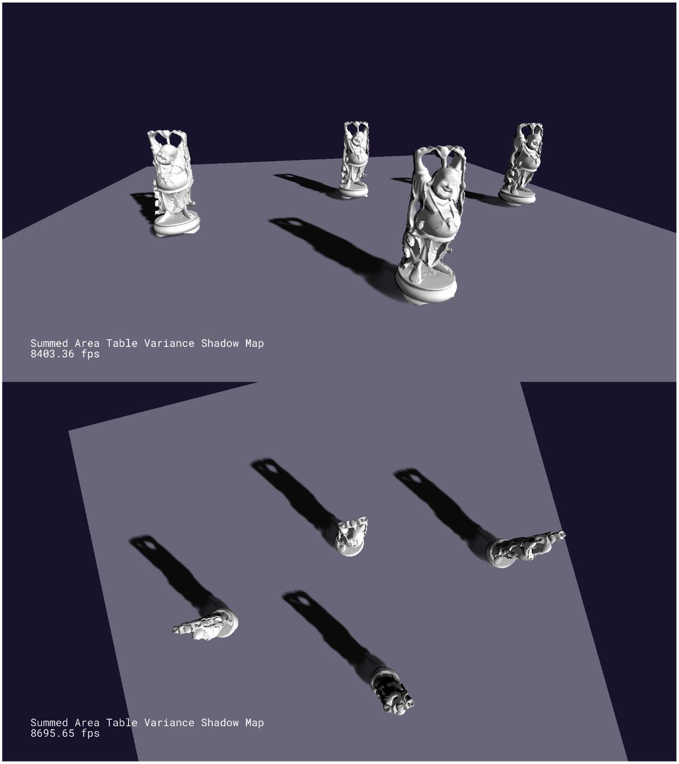
4. Summed Area Table Variance Shadow Map(SATVSM)

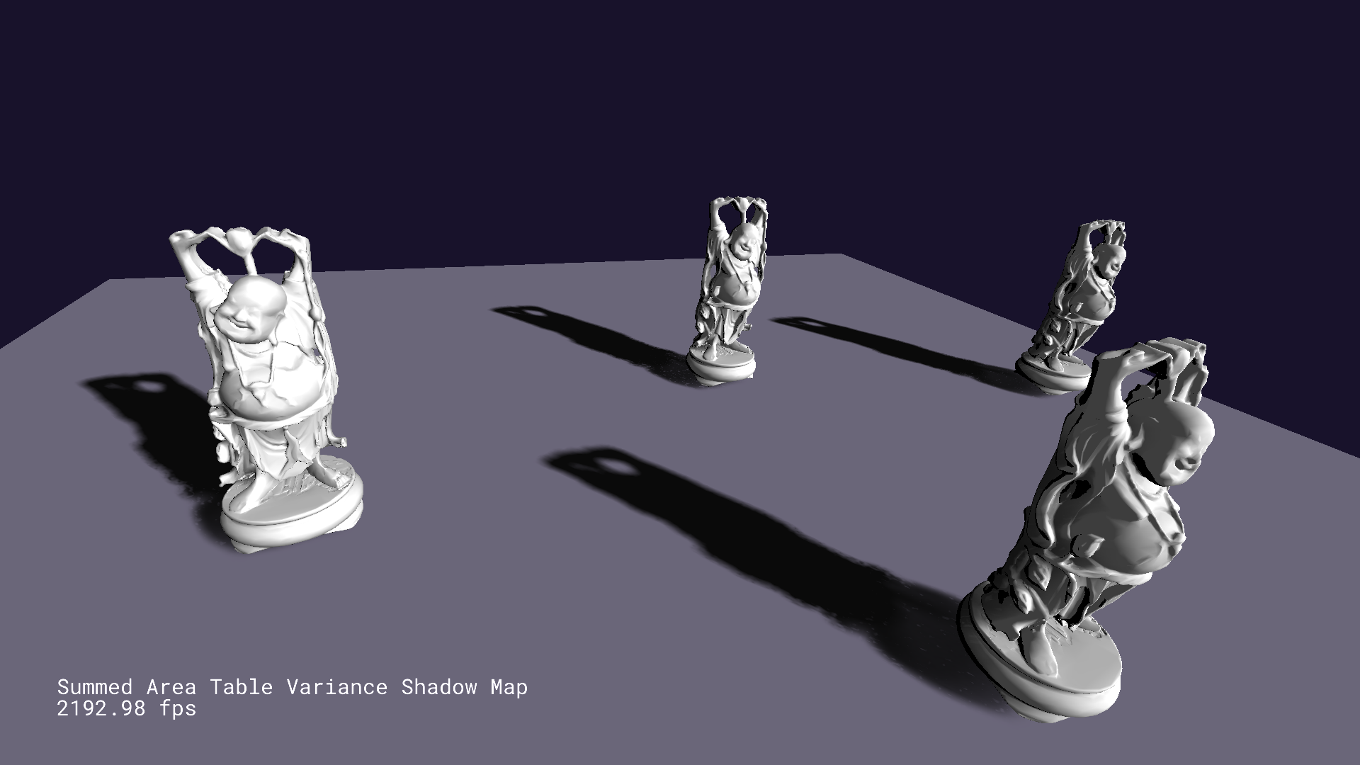
Summed area table makes calculating the summation of a specific range in a texture fast. If this table is generated from the texture moments stored in, shadow calculation by arbitrary area can be accelerated. This table can be created with the method from [3] which is called recursive doubling. Like PCF, a filter size is required when calculating shadows, but this time another method is applied so that the filter size gets increased when the camera is closer to the shadow area to hide artifacts. Besides, bilinear interpolation is considered together while averaging moments in an area. Combined with summed area tables, shadow filtering can be processed in constant time providing plausible soft shadow results.

Light Bleeding

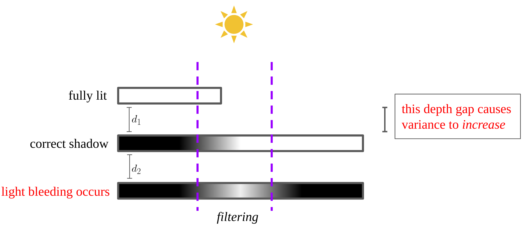
One flaw of variance shadow maps is light bleeding which lights a surface that shadow should be cast on. As shown in the above figure, the big depth gap causes variance $\sigma^2$ to increase, so the upper bound from Cantelli’s inequality is close to $1$ as well. In fact, this artifact gets worse as $d_1/d_2$ is larger. One simple solution for this is to normalize the shadow value with an experimental constant.

  float reduceLightBleeding(in float shadow)
  {
    const float light_bleeding_reduction_amount = 0.18f;
    return clamp( 
      (shadow - light_bleeding_reduction_amount) / (1.0f - light_bleeding_reduction_amount), 
      0.0f, 1.0f 
    );
  }

References

[1] Tutorial 42: Percentage Closer Filtering

[2] Chapter 8. Summed-Area Variance Shadow Maps

[3] Hensley, Justin, Thorsten Scheuermann, Greg Coombe, Montek Singh, and Anselmo Lastra, Fast Summed-Area Table Generation and Its Applications, Computer Graphics Forum 24(3).

Code

https://github.com/emoy-kim/VarianceShadowMaps