Integration Techniques

1. Wallis Formula

In=0π2sinnxdx=0π2cosnxdxIn={  n1nn3n2n5n4    12π2(even n2)  n1nn3n2n5n4    231(odd n3)\begin{aligned} I_n &= \int_0^{\frac{\pi}{2}} \sin^n x dx = \int_0^{\frac{\pi}{2}} \cos^n x dx \\\\ I_n &= \begin{cases} \; \cfrac{n-1}{n} \cdot \cfrac{n-3}{n-2} \cdot \cfrac{n-5}{n-4} \cdot \; \cdots \; \cdot \cfrac{1}{2} \cdot \cfrac{\pi}{2} & (\text{even } n \geq 2)\\\\ \; \cfrac{n-1}{n} \cdot \cfrac{n-3}{n-2} \cdot \cfrac{n-5}{n-4} \cdot \; \cdots \; \cdot \cfrac{2}{3} \cdot 1 & (\text{odd } n \geq 3) \end{cases} \end{aligned}

Imagining the graph of sinx\sin x and cosx\cos x, this identity in the first line seems obvious. Using partial integration, this formula can be derived as follows. In=0π2sinnxdx=0π2sinxsinn1xdx=[cosxsinn1x]0π2+0π2cosx(n1)sinn2xcosxdx=(n1)0π2(1sin2x)sinn2xdx=(n1)0π2sinn2xdx(n1)0π2sinnxdx=(n1)In1(n1)In    In=n1nIn2    I0=0π2sin0xdx=[x]0π2=π2,I1=0π2sinxdx=[cosx]0π2=1    In={  n1nn3n2n5n4    12I0(even n2)  n1nn3n2n5n4    23I1(odd n3)\begin{aligned} I_n &= \int_0^{\frac{\pi}{2}} \sin^n x dx = \int_0^{\frac{\pi}{2}} \sin x \cdot \sin^{n-1} x dx \\ &= \left[ -\cos x \cdot \sin^{n-1} x \right]_0^{\frac{\pi}{2}} + \int_0^{\frac{\pi}{2}} \cos x \cdot (n - 1) \sin^{n-2} x \cdot \cos xdx \\ &= (n - 1) \int_0^{\frac{\pi}{2}} (1 - \sin^2 x) \sin^{n-2} x dx \\ &= (n - 1) \int_0^{\frac{\pi}{2}} \sin^{n-2} x dx - (n - 1) \int_0^{\frac{\pi}{2}} \sin^{n} x dx \\ &= (n - 1) I_{n-1} - (n - 1) I_n \\ \implies I_n &= \cfrac{n-1}{n} I_{n-2} \\ \implies I_0 &= \int_0^{\frac{\pi}{2}} \sin^0 x dx = \left[ x \right]_0^{\frac{\pi}{2}} = \cfrac{\pi}{2}, \quad I_1 = \int_0^{\frac{\pi}{2}} \sin x dx = \left[ -\cos x \right]_0^{\frac{\pi}{2}} = 1 \\\\ \implies I_n &= \begin{cases} \; \cfrac{n-1}{n} \cdot \cfrac{n-3}{n-2} \cdot \cfrac{n-5}{n-4} \cdot \; \cdots \; \cdot \cfrac{1}{2} \cdot I_0 & (\text{even } n \geq 2) \\\\ \; \cfrac{n-1}{n} \cdot \cfrac{n-3}{n-2} \cdot \cfrac{n-5}{n-4} \cdot \; \cdots \; \cdot \cfrac{2}{3} \cdot I_1 & (\text{odd } n \geq 3) \end{cases} \end{aligned}

2. Gamma Function

Γ(n+1)=0exxndx=lima[exxn]0a+n0exxn1dx=n0exxn1dx=nΓ(n)(n>0)=n(n1)Γ(n1)==n!Γ(0)=n!\begin{aligned} \Gamma(n+1) &= \int_0^{\infty} e^{-x} x^n dx \\ &= \lim_{a \to \infty} \left[ -e^{-x} x^n \right]_0^{a} + n \int_0^{\infty} e^{-x} x^{n-1} dx \\ &= n \int_0^{\infty} e^{-x} x^{n-1} dx = n\Gamma(n) \quad (n>0) \\ &= n(n - 1)\Gamma(n - 1) = \cdots = n! \Gamma(0) = n! \end{aligned}

By definition, the gamma function looks like the above. Moreover, by the substitution ex=te^{-x} = t, Γ(n+1)=0exxndx=10+t(lnt)n(1tdt)=0+1(lnt)ndt=0+1(lnx)ndx\begin{aligned} \Gamma(n+1) &= \int_0^{\infty} e^{-x} x^n dx = \int_1^{0+} t (-\ln t)^n \left( -\frac{1}{t} dt \right) \\ &= \int_{0+}^1 (-\ln t)^n dt = \int_{0+}^1 (-\ln x)^n dx \end{aligned}

The following two properties are worth remembering.

  • Γ(n)Γ(1n)=πsinnπ  \Gamma(n) \Gamma(1-n) = \cfrac{\pi}{\sin n \pi}\;,
  • Γ(1)=0exlnxdx\Gamma'(1) = \displaystyle \int_0^{\infty} e^{-x} \ln x dx.

3. Heaviside Cover-Up Method

The Heaviside cover-up method is a technique to make a partial-fractions decomposition of a rational function f(x)/g(x)f(x)/g(x) whenever the denominator can be factored into distinct linear factors. f(x)g(x)=f(x)(xr1)(xr2)(xrn)=A1xr1+A2xr2++Anxrn    A1=f(r1)(r1r2)(r1r3)(r1rn),A2=f(r2)(r2r1)(r2r3)(r2rn),An=f(rn)(rnr1)(rnr2)(rnrn1)\begin{aligned} \cfrac{f(x)}{g(x)} &= \cfrac{f(x)}{(x - r_1)(x - r_2)\cdots(x - r_n)} = \cfrac{A_1}{x - r_1} + \cfrac{A_2}{x - r_2} + \cdots + \cfrac{A_n}{x - r_n} \\\\ \implies A_1 &= \cfrac{f(r_1)}{(r_1 - r_2)(r_1 - r_3)\cdots(r_1 - r_n)}, \\ A_2 &= \cfrac{f(r_2)}{(r_2 - r_1)(r_2 - r_3)\cdots(r_2 - r_n)}, \\ &\vdots \\ A_n &= \cfrac{f(r_n)}{(r_n - r_1)(r_n - r_2)\cdots(r_n - r_{n-1})} \end{aligned}

4. Integrals involving ax2+bx+c\sqrt{ax^2 + bx + c}

When the integrands are functions of xx and ax2+bx+c\sqrt{ax^2 + bx + c}, the following substitution method is useful. Let α\alpha and β\beta be the roots of ax2+bx+cax^2 + bx + c such that α<β\alpha < \beta. {  a>0    {  D>0    a(xα)xβ=t  D<0    ax2+bx+c=tax  a<0    xαβx=t\begin{aligned} \begin{cases} \; a > 0 & \implies & \begin{cases} \; D > 0 & \implies & \sqrt{\cfrac{a(x - \alpha)}{x - \beta}} = t \\\\ \; D < 0 & \implies & \sqrt{ax^2 + bx + c} = t - \sqrt{a}x \end{cases} \\\\ \; a < 0 & \implies & \sqrt{\cfrac{x - \alpha}{\beta - x}} = t \end{cases} \end{aligned}

Note that DD is the discriminant of ax2+bx+cax^2 + bx + c. After setting as above, both sides should be squared to make the form of x=f(t)x = f(t).

5. Powers of Trigonometric Integrals

The following are indefinite integrals of powers of sinx\sin x and cosx\cos x. In=sinnxdx=sinxsinn1xdx=cosxsinn1x(cosx)(n1)sinn2xcosxdx=cosxsinn1x+(n1)sinn2x(1sin2x)dx=cosxsinn1x+(n1)sinn2xsinnxdx=cosxsinn1x+(n1)(In2In)    In=sinnxdx=1nsinn1xcosx+n1nIn2    Jn=cosnxdx=1ncosn1xsinx+n1nJn2\begin{aligned} I_n &= \int \sin^n x dx = \int \sin x \cdot \sin^{n-1} x dx \\ &= -\cos x \cdot \sin^{n-1} x - \int (-\cos x) (n - 1) \sin^{n-2} x \cdot \cos xdx \\ &= -\cos x \cdot \sin^{n-1} x + (n - 1) \int \sin^{n-2} x (1 - \sin^2 x)dx \\ &= -\cos x \cdot \sin^{n-1} x + (n - 1) \int \sin^{n-2} x - \sin^n xdx \\ &= -\cos x \cdot \sin^{n-1} x + (n - 1) (I_{n-2} - I_n) \\\\ \implies I_n &= \int \sin^n x dx = -\cfrac{1}{n} \sin^{n-1}x \cdot \cos x + \cfrac{n-1}{n} I_{n-2} \\ \implies J_n &= \int \cos^n x dx = -\cfrac{1}{n} \cos^{n-1}x \cdot \sin x + \cfrac{n-1}{n} J_{n-2} \end{aligned}

The following are indefinite integrals of powers of tanx\tan x and cotx\cot x. In=tannxdx=tann2xtan2xdx=tann2x(sec2x1)dx=tann2xsec2xdxtann2xdx=1n1tann1xIn2    In=tannxdx=1n1tann1xIn2    Jn=cotnxdx=1n1cotn1xJn2\begin{aligned} I_n &= \int \tan^n x dx = \int \tan^{n-2} x \cdot \tan^{2} x dx = \int \tan^{n-2} x (\sec^2 x - 1)dx \\ &= \int \tan^{n-2} x \sec^2 xdx - \int \tan^{n-2} xdx = \cfrac{1}{n-1} \tan^{n-1} x - I_{n-2} \\ \implies I_n &= \int \tan^n x dx = \cfrac{1}{n-1} \tan^{n-1}x - I_{n-2} \\ \implies J_n &= \int \cot^n x dx = -\cfrac{1}{n-1} \cot^{n-1}x - J_{n-2} \end{aligned}

The following are indefinite integrals of powers of secx\sec x and cscx\csc x. In=secnxdx=sec2xsecn2xdx=tanxsecn2x(n2)secn2xtan2xdx=tanxsecn2x(n2)secn2x(sec2x1)dx=tanxsecn2x(n2)secnxdx+(n2)secn2xdx=tanxsecn2x(n2)In+(n2)In2    In=secnxdx=1n1secn2xtanx+n2n1In2    Jn=cscnxdx=1n1cscn2xcotx+n2n1Jn2\begin{aligned} I_n &= \int \sec^n x dx = \int \sec^2 x \cdot \sec^{n-2} x dx \\ &= \tan x \cdot \sec^{n-2} x - \int (n - 2) \sec^{n-2} x \cdot \tan^2 xdx \\ &= \tan x \cdot \sec^{n-2} x - (n - 2) \int \sec^{n-2} x (\sec^2 x - 1)dx \\ &= \tan x \cdot \sec^{n-2} x - (n - 2) \int \sec^{n} xdx + (n - 2) \int \sec^{n-2} xdx \\ &= \tan x \cdot \sec^{n-2} x - (n - 2) I_n + (n - 2) I_{n-2} \\\\ \implies I_n &= \int \sec^n x dx = \cfrac{1}{n-1} \sec^{n-2}x \cdot \tan x + \cfrac{n-2}{n-1} I_{n-2} \\ \implies J_n &= \int \csc^n x dx = -\cfrac{1}{n-1} \csc^{n-2}x \cdot \cot x + \cfrac{n-2}{n-1} J_{n-2} \end{aligned}

6. Definite Integrals Involving Trigonometric Functions

The following formulas are worth remembering.

  • 0πsinmxsinnxdx={  0(mn integers)  π2(m=n integers)\displaystyle \int_0^{\pi} \sin mx \cdot \sin nx dx = \begin{cases} \; 0 & (m \ne n \text{ integers}) \\ \; \cfrac{\pi}{2} & (m = n \text{ integers}) \end{cases},
  • 0πcosmxcosnxdx={  0(mn integers)  π2(m=n integers)\displaystyle \int_0^{\pi} \cos mx \cdot \cos nx dx = \begin{cases} \; 0 & (m \ne n \text{ integers}) \\ \; \cfrac{\pi}{2} & (m = n \text{ integers}) \end{cases},
  • 0πsinmxcosnxdx={  0(integers m and n, even m+n)  2mm2n2(integers m and n, odd m+n)\displaystyle \int_0^{\pi} \sin mx \cdot \cos nx dx = \begin{cases} \; 0 & (\text{integers } m \text{ and } n, \text{ even } m + n) \\ \; \cfrac{2m}{m^2-n^2} & (\text{integers } m \text{ and } n, \text{ odd } m + n) \end{cases},
  • 0sinmxxdx={  0(m=0)  π2(m>0)  π2(m<0)\displaystyle \int_0^{\infty} \cfrac{\sin mx}{x} dx = \begin{cases} \; 0 & (m = 0) \\ \; \cfrac{\pi}{2} & (m > 0) \\ \; -\cfrac{\pi}{2} & (m < 0) \end{cases},
  • 0sin2mxx2dx=mπ2\displaystyle \int_0^{\infty} \cfrac{\sin^2 mx}{x^2} dx = \cfrac{m\pi}{2},
  • 0tanxxdx=π2\displaystyle \int_0^{\infty} \cfrac{\tan x}{x} dx = \cfrac{\pi}{2},
  • 01sin1xxdx=π2ln2\displaystyle \int_0^1 \cfrac{\sin^{-1} x}{x} dx = \cfrac{\pi}{2} \ln 2,
  • 0πxf(sinx)dx=π20πf(sinx)dx\displaystyle \int_0^{\pi} x f(\sin x) dx = \cfrac{\pi}{2} \int_0^{\pi} f(\sin x) dx.

7. When the Denominator of Integrand Includes Trigonometric Functions

Approaches for this type of integration differ on whether the denominator of integrand is a form of linear trigonometric function or quadratic trigonometric function. Note that it is better to use the way for the quadratic trigonometric function when the denominator of the integrand includes tanx\tan x. Even in the case of the double-angle form, using the approach for the quadratic trigonometric function is proper. {  tanx2=t    sinx=2t1+t2,cosx=1t21+t2,tanx=2t1t2  tanx=t    sinx=t1+t2,cosx=11+t2\begin{aligned} \begin{cases} \; \tan \cfrac{x}{2} = t & \implies \sin x = \cfrac{2t}{1+t^2}, \quad \cos x = \cfrac{1-t^2}{1+t^2}, \quad \tan x = \cfrac{2t}{1-t^2} \\\\ \; \tan x = t & \implies \sin x = \cfrac{t}{\sqrt{1+t^2}}, \quad \cos x = \cfrac{1}{\sqrt{1+t^2}} \end{cases} \end{aligned}

sinx\sin x and cosx\cos x for each case can be derived by drawing the right triangle satisfying tanx\tan x for tt.

8. Cauchy-Schwarz Inequality

For two functions ff and gg, if these functions are continuous in [a,b][a, b], the following inequalities hold.

  • (abf(x)g(x)dx)2(abf(x)2dx)(abg(x)2dx)\left( \displaystyle \int_a^b f(x) g(x) dx \right)^2 \leq \left( \displaystyle \int_a^b f(x)^2 dx \right) \left( \displaystyle \int_a^b g(x)^2 dx \right),
  • (abf(x)dx)2abf(x)2dx\left( \displaystyle \int_a^b f(x) dx \right)^2 \leq \displaystyle \int_a^b f(x)^2 dx.

9. Odd & Even Functions

By definition, a function f(x)f(x) is called the odd function when f(x)=f(x)f(-x) = -f(x), or is called the even function when f(x)=f(x)f(-x) = f(x). These functions have the following properties.

  • Even function ×\times Even function     \implies Even function
  • Odd function ×\times Odd function     \implies Even function
  • Even function ×\times Odd function     \implies Odd function
  • Even function ++ Even function     \implies Even function
  • Odd function ++ Odd function     \implies Odd function
  • Even function ++ Odd function     \implies No Rule
  • Derivative of an Even function     \implies Odd function
  • Derivative of an Odd function     \implies Even function

10. Simpson’s Rule

Simpson’s rule is the approximation for definite integrals based upon a quadratic interpolation. First, for three real numbers x1x_1, x2x_2, and x3x_3 such that x3x2=x2x1=hx_3 - x_2 = x_2 - x_1 = h and x1<x2<x3x_1 < x_2 < x_3, the integration of ax2+bx+cax^2 + bx + c in [x1,x3][x_1, x_3] can be calculated as follows. Note that yi=axi2+bxi+cy_i = ax_i^2 + bx_i + c. x1x3ax2+bx+c  dx=[ax33+bx22+cx]x1x3=a(x33x13)3+b(x32x12)2+c(x3x1)=x3x16(2a(x12+x1x3+x32)+3b(x1+x3)+6c)=2h6((ax12+bx1+c)+(ax32+bx3+c)+a(x1+x3)2+2b(x1+x3)+4c)=h3(y1+y3+a(2x2)2+2b(2x2)+4c)=h3(y1+y3+4y2)\begin{aligned} &\int_{x_1}^{x_3} ax^2 + bx + c \; dx = \left[ \cfrac{ax^3}{3} + \cfrac{bx^2}{2} + cx \right]_{x_1}^{x_3} = \cfrac{a(x_3^3 - x_1^3)}{3} + \cfrac{b(x_3^2 - x_1^2)}{2} + c(x_3 - x_1) \\ &= \cfrac{x_3 - x_1}{6} \left( 2a (x_1^2 + x_1 x_3 + x_3^2) + 3b (x_1 + x_3) + 6c \right) \\ &= \cfrac{2h}{6} \left( (ax_1^2 + bx_1 + c) + (a x_3^2 + b x_3 + c) + a(x_1 + x_3)^2 + 2b(x_1 + x_3) + 4c \right) \\ &= \cfrac{h}{3} \left( y_1 + y_3 + a(2x_2)^2 + 2b(2x_2) + 4c \right) = \cfrac{h}{3} \left( y_1 + y_3 + 4y_2 \right) \end{aligned}

Now, to integrate a function f(x)f(x) in [a,b][a, b], the above result can be applied. Let h=(ba)/2nh = (b - a)/2n, x0=ax_0 = a, x2n=bx_{2n} = b, and yi=f(xi)y_i = f(x_i). Then, the approximation of the integration of f(x)f(x) is abf(x)dxh3(y0+4y1+y2)+h3(y2+4y3+y4)++h3(y2n2+4y2n1+y2n)=h3(y0+4(y1+y3++y2n1)+2(y2+y4++y2n2)+y2n)\begin{aligned} \int_{a}^{b} f(x) dx &\approx \cfrac{h}{3} \left( y_0 + 4y_1 + y_2 \right) + \cfrac{h}{3} \left( y_2 + 4y_3 + y_4 \right) + \cdots + \cfrac{h}{3} \left( y_{2n-2} + 4y_{2n-1} + y_{2n} \right) \\ &= \cfrac{h}{3} \left( y_0 + 4(y_1 + y_3 + \cdots + y_{2n-1}) + 2(y_2 + y_4 + \cdots + y_{2n-2}) + y_{2n} \right) \end{aligned}

This formula is called Simpson’s rule, and if f(x)f(x) is a four times-differentiable function, then the error EE in the approximation is E(ba)5180n4max(f(4)(ξ))(aξb)\begin{aligned} E \leq \cfrac{(b - a)^5}{180 n^4} \max(\vert f^{(4)}(\xi) \vert) \quad (a \leq \xi \leq b) \end{aligned}

11. Important Power Series

  • 11x=1+x+x2+=n=0xn(x<1)  \cfrac{1}{1-x} = 1 + x + x^2 + \cdots = \displaystyle \sum_{n=0}^{\infty} x^n \quad (\vert x \vert < 1) \;,
  • ex=1+x+x22!+=n=0xnn!  e^x = 1 + x + \cfrac{x^2}{2!} + \cdots = \displaystyle \sum_{n=0}^{\infty} \cfrac{x^n}{n!} \;,
  • sinx=xx33!+x55!=n=0(1)nx2n+1(2n+1)!  \sin x = x - \cfrac{x^3}{3!} + \cfrac{x^5}{5!} - \cdots = \displaystyle \sum_{n=0}^{\infty} (-1)^n \cfrac{x^{2n+1}}{(2n+1)!} \;,
  • cosx=1x22!+x44!=n=0(1)nx2n(2n)!  \cos x = 1 - \cfrac{x^2}{2!} + \cfrac{x^4}{4!} - \cdots = \displaystyle \sum_{n=0}^{\infty} (-1)^n \cfrac{x^{2n}}{(2n)!} \;,
  • ln(1+x)=xx22+x33=n=1(1)n+1xnn(1<x1)  \ln (1 + x) = x - \cfrac{x^2}{2} + \cfrac{x^3}{3} - \cdots = \displaystyle \sum_{n=1}^{\infty} (-1)^{n+1} \cfrac{x^{n}}{n} \quad (-1 < x \leq 1) \;,
  • sin1x=x+123x3+13245x5+=n=0(2n)!22n(n!)2x2n+12n+1(x1)  \sin^{-1} x = x + \cfrac{1}{2 \cdot 3}x^3 + \cfrac{1 \cdot 3}{2 \cdot 4 \cdot 5}x^5 + \cdots = \displaystyle \sum_{n=0}^{\infty} \cfrac{(2n)!}{2^{2n}(n!)^2} \cfrac{x^{2n+1}}{2n+1} \quad (\vert x \vert \leq 1) \;,
  • cos1x=π2(x+123x3+13245x5+)=π2n=0(2n)!22n(n!)2x2n+12n+1(x1)  \cos^{-1} x = \cfrac{\pi}{2} - \left( x + \cfrac{1}{2 \cdot 3}x^3 + \cfrac{1 \cdot 3}{2 \cdot 4 \cdot 5}x^5 + \cdots \right) = \cfrac{\pi}{2} - \displaystyle \sum_{n=0}^{\infty} \cfrac{(2n)!}{2^{2n}(n!)^2} \cfrac{x^{2n+1}}{2n+1} \quad (\vert x \vert \leq 1) \;,
  • tan1x=xx33+x55=n=0(1)nx2n+12n+1(x1)  \tan^{-1} x = x - \cfrac{x^3}{3} + \cfrac{x^5}{5} - \cdots = \displaystyle \sum_{n=0}^{\infty} (-1)^n \cfrac{x^{2n+1}}{2n+1} \quad (\vert x \vert \leq 1) \;,
  • 1x=1x2x28x316=n=0(1)nxn(12n)(x<1)  \sqrt{1-x} = 1 - \cfrac{x}{2} - \cfrac{x^2}{8} - \cfrac{x^3}{16} - \cdots = \displaystyle \sum_{n=0}^{\infty} (-1)^n x^n \binom{\frac{1}{2}}{n} \quad (\vert x \vert < 1) \;,
  • sinhx=x+x33!+x55!+=n=0x2n+1(2n+1)!  \sinh x = x + \cfrac{x^3}{3!} + \cfrac{x^5}{5!} + \cdots = \displaystyle \sum_{n=0}^{\infty} \cfrac{x^{2n+1}}{(2n+1)!} \;,
  • coshx=1+x22!+x44!+=n=0x2n(2n)!  \cosh x = 1 + \cfrac{x^2}{2!} + \cfrac{x^4}{4!} + \cdots = \displaystyle \sum_{n=0}^{\infty} \cfrac{x^{2n}}{(2n)!} \;.

12. Shell Integration

This is a method for calculating the volume of a solid of revolution when integrating along an axis perpendicular to the axis of revolution. If a function y=f(x)y = f(x) in [a,b][a, b] is rotating around the line x=mx = m, then the volume is V=xnearxfar2π(xm)f(x)dx\begin{aligned} V = \int_{x_{\text{near}}}^{x_{\text{far}}} 2\pi (x - m) f(x) dx \end{aligned}

where xnearx_{\text{near}} and xfarx_{\text{far}} are each the closer point and the farther point to the rotation axis among aa and bb. Similarly, If a function x=f(y)x = f(y) in [c,d][c, d] is rotating around the line y=ny = n, then the volume is V=ynearyfar2π(yn)f(y)dy\begin{aligned} V = \int_{y_{\text{near}}}^{y_{\text{far}}} 2\pi (y - n) f(y) dy \end{aligned}

where yneary_{\text{near}} and yfary_{\text{far}} are each the closer point and the farther point to the rotation axis among cc and dd. An example can be found here.

13. Pappus’s Centroid Theorem

The volume of a solid obtained by revolving a plane region RR about a line ll is V=2πρA\begin{aligned} V = 2\pi \rho A \end{aligned}

where ρ\rho is the distance from ll to the geometric centroid of RR and AA is the area of RR. This theorem does not require integration to get a volume, but it might be hard to find the geometric centroid of RR.

14. Center of Mass

Given that nn particles PiP_i whose each with mass mim_i that are located to coordinates Pi(xi,yi,zi)P_i(x_i, y_i, z_i), the center of mass (xc,yc,zc)(x_c, y_c, z_c) is (xc,yc,zc)=1i=1nmi(i=1nmixi,i=1nmiyi,i=1nmizi)\begin{aligned} (x_c, y_c, z_c) = \cfrac{1}{\displaystyle \sum_{i=1}^n m_i} \left( \sum_{i=1}^n m_i x_i, \sum_{i=1}^n m_i y_i, \sum_{i=1}^n m_i z_i \right) \end{aligned}

If the mass distribution is continuous, for the total mass MM, M(xc,yc,zc)=(xmdm,ymdm,zmdm)\begin{aligned} M(x_c, y_c, z_c) = \left( \int x_m dm, \int y_m dm, \int z_m dm \right) \end{aligned}

where (xm,ym,zm)(x_m, y_m, z_m) is the center of the infinitesimal mass dmdm. The key property related to this is for a fragmented shape SS on a plane. Assume that SS is fragemented into S1,S2,S_1, S_2, \cdots. Also, let the distances from an axis ll to each fragment be d1,d2,d_1, d_2, \cdots. Then, the center of SS is located at a distance dd from ll such that Sd=S1d1+S2d2+\begin{aligned} Sd = S_1 d_1 + S_2 d_2 + \cdots \end{aligned}

15. Double Integral

The following are techniques to calculate a double integral.

16. Curved Surface Area

SurfaceArea

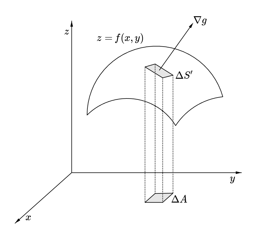
To calculate the surface area defined by z=f(x,y)z = f(x, y), let this area be SS and AA be the projected area of SS on xyxy-plane. Then, ΔA=ΔxΔy\Delta A = \Delta x \Delta y. Now, considering the right rectangle prism with ΔA\Delta A as its base, this prism slices the surface so that the sliced curved surface area is ΔS\Delta S. For a point PP within the ΔS\Delta S region, the tangent plane at PP slices the right rectangle prism so that the sliced plane area is ΔS\Delta S'. So, it implies that the projection of ΔS\Delta S' on xyxy-plane is ΔA\Delta A. The normal vector of this tangent plane can be obtained from the gradient g\nabla g where g(x,y,z)=zf(x,y)g(x, y, z) = z - f(x, y). Moreover, the angle θ\theta between this tangent plane and xyxy-plane can be computed by the dot product of their normal vectors.
ΔA=ΔScosθ,g=(fx,  fy,  1)=(fx,fy,1)    cosθ=g(0,0,1)g=11+fx2+fy2    ΔS=1+fx2+fy2ΔxΔy\begin{aligned} &\Delta A = \Delta S' \cos \theta, \quad \nabla g = \left( -\cfrac{\partial f}{\partial x}, \; -\cfrac{\partial f}{\partial y}, \; 1 \right) = (-f_x, -f_y, 1) \\ \implies &\cos \theta = \cfrac{\nabla g \cdot (0, 0, 1)}{\Vert \nabla g \Vert} = \cfrac{1}{\sqrt{1 + f_x^2 + f_y^2}} \implies \Delta S' = \sqrt{1 + f_x^2 + f_y^2} \Delta x \Delta y \end{aligned}

Since ΔS\Delta S' is approximately same as ΔS\Delta S when Δx\Delta x and Δy\Delta y approach 00, the curved surface area of f(x,y)f(x, y) whose projection on xyxy-plane is defined in a region DD is calculated as follows. limΔx,Δy0ΔSΔS=1    S=D1+fx2+fy2  dxdy\begin{aligned} \lim_{\Delta x, \Delta y \to 0} \cfrac{\Delta S'}{\Delta S} = 1 \implies S = \iint_D \sqrt{1 + f_x^2 + f_y^2} \; dx dy \end{aligned}


© 2024. All rights reserved.