Coordinates Transformation of a Double Integral

• Coordinates Transformation
• Polar Coordinate System
• Ellipse to Rectangle
• Lozenge to Square
• Application

Coordinates Transformation

If a double integral is still tricky even after considering Fubini’s theorem, the next step to consider is the transformation of the coordinate system. More specifically, a region $A$ of $xy$-plane can be transformed to a region $B$ of $uv$-plane by $x = f(u, v)$ and $y = g(u, v)$. A function $\phi(x, y)$ defined in $A$ can be viewed as a function $\phi(f(u, v), g(u, v))$ defined in $B$. $$\begin{aligned} \iint_A \phi(x, y)dxdy = \iint_B \phi(f(u, v), g(u, v)) \left \vert \cfrac{\partial (x, y)}{\partial (u, v)} \right \vert dudv \end{aligned}$$

where $\left \vert \partial (x, y) / \partial (u, v) \right \vert$ is the Jacobian determinant mentioned in this note. That is, this Jacobian determinant compensates for the difference caused by the transformation. So, the relationship between $A$ and $B$ is that $A = \vert J \vert B \iff B = A \vert J^{-1} \vert$. The inverse of the Jacobian is effective when the arrangement such as $x = f(u, v)$ and $y = g(u, v)$ seems hard.

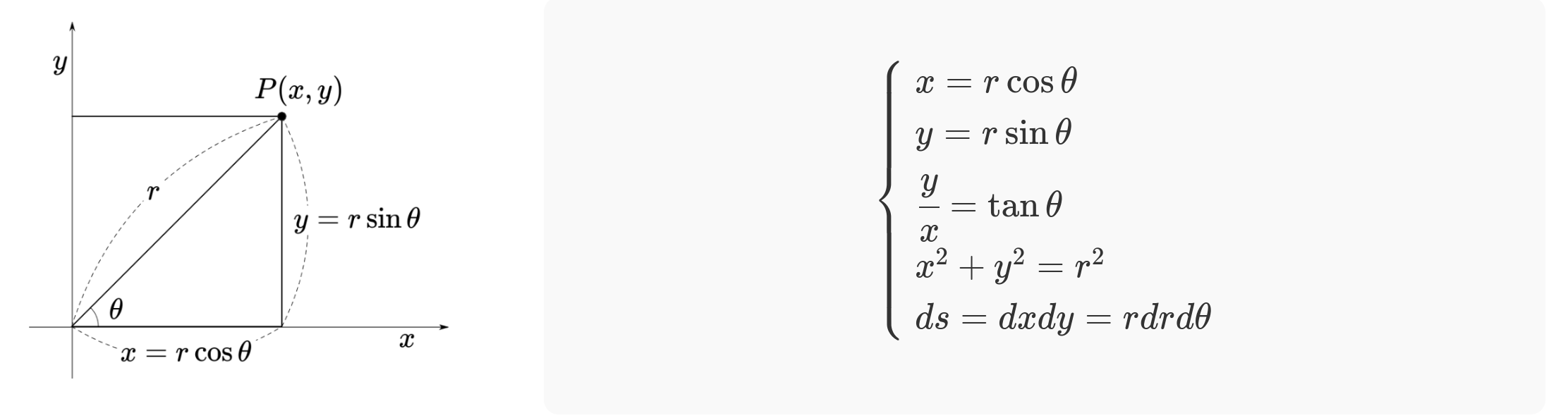
Polar Coordinate System

$$\begin{aligned} \iint_\text{ortho} f(x, y)dxdy = \iint_\text{polar} f(r, \theta) r drd\theta \end{aligned}$$

The first to consider is the transformation of the orthogonal coordinate system to the polar coordinate system. The relationship between the two coordinate systems is as follows.

Note that $ds$ can be obtained from the Jacobian determinant to compensate for the difference caused by the transformation. $$\begin{aligned} ds = dx dy = \left \vert \cfrac{\partial (x, y)}{\partial (r, \theta)} \right \vert dr d\theta = \left \vert \begin{array}{cc} \frac{\partial (r \cos \theta)}{\partial r} & \frac{\partial (r \cos \theta)}{\partial \theta} \\ \frac{\partial (r \sin \theta)}{\partial r} & \frac{\partial (r \sin \theta)}{\partial \theta} \end{array} \right \vert dr d\theta = \left \vert \begin{array}{cc} \cos \theta & -r \sin \theta \\ \sin \theta & r \cos \theta \end{array} \right \vert dr d\theta = r dr d\theta \end{aligned}$$

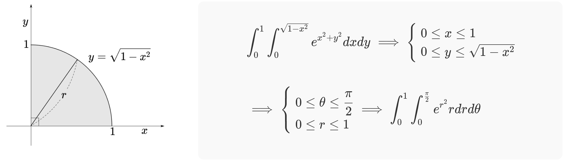
For example, the following double integral can be transformed into the polar coordinate system.

The following two formulae are worth remembering since they are often used in the polar coordinate system.

• $\displaystyle \int_0^{\infty} e^{-kx^2} dx = \cfrac{\sqrt{\pi}}{2\sqrt{k}} \;$,

• $\displaystyle \int_0^{\infty} \cfrac{e^{-kx}}{\sqrt{x}} dx = \cfrac{\sqrt{\pi}}{\sqrt{k}} \;$.

Ellipse to Rectangle

This transformation may also make it easy to calculate a double integral.

• Ellipse to Circle $\implies x = au$ and $y = bv$
• Circle to Rectangle $\implies u = r \cos \theta$ and $v = r \sin \theta$

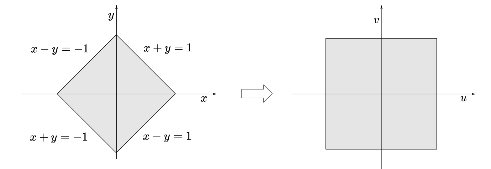
Lozenge to Square

When transforming a coordinate system, it is sometimes hard to determine the interval of integration. In this case, the lozenge transformation by the substitution method may be quite useful.

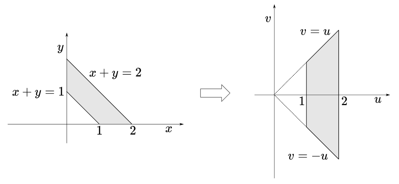
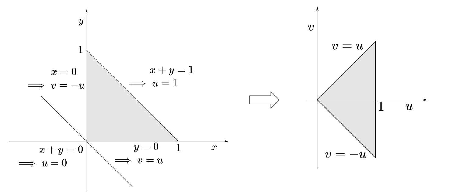
Case 1. $x + y = u$ and $x - y = v$

This substitution can be arranged as follows. $$\begin{aligned} x = \cfrac{u + v}{2}, \quad y = \cfrac{u - v}{2} \implies \vert J \vert = \left \vert \begin{array}{cc} \frac{1}{2} & \frac{1}{2} \\ \frac{1}{2} & -\frac{1}{2} \end{array} \right \vert = -\cfrac{1}{2} \end{aligned}$$

The following list shows that a function $f(x, y)$ defined in a region $D$ transforms into a function $f(u, v)$. When graphing the range of variables, it is better that a few points can be directly put into to figure out where they are transformed. In this case, for example, $(0, 0) \to (0, 0)$, $(1, 0) \to (1, 1)$, and $(0, 1) \to (1, -1)$.

$$\begin{aligned} \iint_D f(x, y)dxdy = \int_{-1}^{1} \int_{-1}^{1} f(u, v) \cfrac{1}{2} dvdu \end{aligned}$$

---

$$\begin{aligned} \iint_D f(x, y)dxdy = \int_{0}^{1} \int_{-u}^{u} f(u, v) \cfrac{1}{2} dvdu \end{aligned}$$

---

$$\begin{aligned} \iint_D f(x, y)dxdy = \int_{1}^{2} \int_{-u}^{u} f(u, v) \cfrac{1}{2} dvdu \end{aligned}$$

---

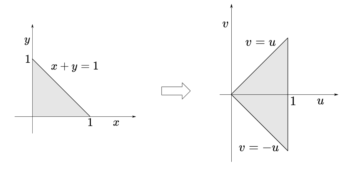
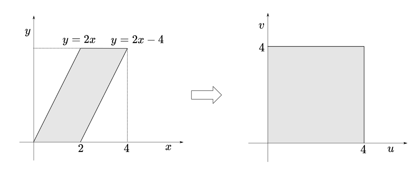
Case 2. $2x - y = u$ and $y = v$

This substitution can be arranged as follows. $$\begin{aligned} x = \cfrac{u + v}{2}, \quad y = v \implies \vert J \vert = \left \vert \begin{array}{cc} \frac{1}{2} & \frac{1}{2} \\ 0 & 1 \end{array} \right \vert = \cfrac{1}{2} \end{aligned}$$

Similarly with case 1, a function $f(x, y)$ defined in a region $D$ transforms into a function $f(u, v)$ as follows.

$$\begin{aligned} \iint_D f(x, y)dxdy = \int_{0}^{4} \int_{0}^{4} f(u, v) \cfrac{1}{2} dvdu \end{aligned}$$

Application

Calculate $$\begin{aligned} \int_{0}^{1} \int_{0}^{1-x} e^{\frac{y}{x+y}} dydx \end{aligned}$$

---

Let $x + y = u$ and $x - y = v$. Then, the upper and lower bounds can be obtained to set the interval of integration.

• When $y=1-x$, $u=x+y=1$. As such, $0 \leq u \leq 1$.
• When $x = 0$, $v = -u$.
• When $y = 0$, $v = u$.

$$\begin{aligned} \int_{0}^{1} \int_{0}^{1-x} e^{\frac{y}{x+y}} dydx = \cfrac{1}{2} \int_{0}^{1} \int_{-u}^{u} e^{\frac{u-v}{2u}} dvdu = \int_{0}^{1} \left[ -u e^{\frac{u-v}{2u}} \right]_{-u}^u du = \int_{0}^{1} u(e-1) du = \cfrac{e-1}{2} \end{aligned}$$