Ambient Occlusion

• 1. Dynamic Ambient Occlusion [1]
  • Surface Elements
  • Surface Elements Tree
  • Shadow Approximation
  • Modulation
  • Result
• 2. High Quality Ambient Occlusion [2]
  • Disks
  • Occlusion Tree
  • Shadow Approximation
  • Robust Solution
  • Result
• References
• Code

The ambient occlusion is about calculation the amount of ambient lighting for each point on an object. [1] and [2] suggest algorithms for this based on disks.

1. Dynamic Ambient Occlusion [1]

Surface Elements

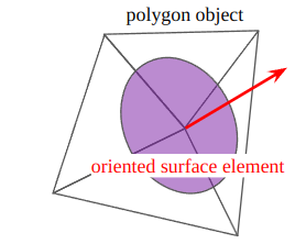
This algorithm converts polygon data from an object to surface elements, which are created per-vertex. Note that only triangle polyon data are considered in this project. Each surface element has its own position, normal, and area information. Most vertices are not isolated, which means they may share multiple faces. To create a surface element, therefore, normals and area information should be averaged by how many faces are surrounding each vertex. While Heron’s formula for the area of a triangle is suggested from this algorithm, it can be calculated by using cross product as well because all vertices have already known.

Surface Elements Tree

After creating surface elements from all the vertices, a tree should be built from these elements. Importantly, these elements are going to be leaf nodes of the tree, which means that some other parent nodes are added to build this tree. It is important in that the time complexity of the tree traversal becomes efficient since all leaf nodes do not need to be searched to calculate ambient occlusion.

At first, surface elements from all the vertices take a kind of ID from texture coordinates. These ID and texture coordinates acts as a separator to build a tree. Once listing nodes with the same ID, a tree is built with their texture coordinates. After building trees for all ID, these trees can be combined into one big tree. In this process, the existing surface elements from all the vertices become leaf nodes and their parent nodes are created whose position/normal/area information are calculated from their children. To be specific, while position and normal are the average of their children, the area is the sum of their children.

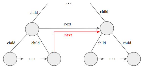
Once the big one tree is built, the new next link should be set as the figure above. The key point is that the next link of the last child should point to the next of its parent. These links make the tree traversal from the root complete if the child-first order is applied. In a shader for calculating ambient occlusion, this tree is searched from the root by pixel.

Shadow Approximation

This algorithm calculates disk-to-disk ambient occlusion. For each vertex, the corresponding surface element disk, receiver, calculates ambient occlusion for all the other surface elements, emitters. Thanks to the surface elements tree structure, the complete traversal may not be required if the parent nodes can give the right enough information on behalf of their children. Once the receiver and emitter are determined, the shadow approximation can be calculated between theses, and all shadow values from emitters are accumulated. The formula of shadow approximation [1] suggests is as follows: $$\begin{aligned} \overbrace{\left(1 - \frac{d}{\sqrt{A/\pi + d^2}}\right)}^{\text{part A}} \cdot \underbrace{s(\cos \theta_E)}_{\text{part B}} \cdot \underbrace{s(\alpha \cos \theta_R)}_{\text{part C}} \end{aligned}$$

Note that this formula is different from Equation 14-1 in [1]. However, SolidAngle() explains in the different way in [3].

where $s(x) = \max(0, \min(1, x))$ and $\alpha$ is an experimental constant, which is $4$ in this project. This formula is based on the solid angle. To try to understand why [1] suggets this formula, I separated this into three parts. I think that the part A is the one which is related to the solid angle. Since disks are oriented, receiver and emitter may not be parallel. However, it seems that the part A is based on the assumption these are parallel. After that, this assumption is relieved going through the part B and C.

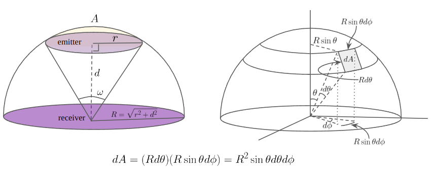
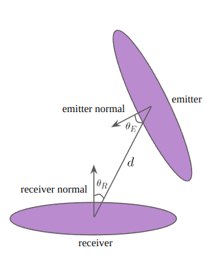
Accordingly, assuming that the receiver and emitter disks are parralel, the solid angle $\omega$ can be calculated from the hemisphere containing the emitter as shown the above figure. Let $r$ and $d$ be the radius of the emitter and the distance between the receiver and the emitter. Then the radius of this hemisphere $R$ should be $\sqrt{r^2 + d^2}$ and the spherical surface area $A$ projected outward onto the surface of this hemisphere from the emitter can be represented as follows: $$\begin{aligned} A &= \int dA = \int_{0}^{2\pi} \int_{0}^{\tan^{-1}{(r/d)}} R^2 \sin{\theta} d\theta d\phi \\ &= \int_{0}^{2\pi} R^2 \lbrack -\cos{\theta} \rbrack_{0}^{\tan^{-1}(r/d)} d\phi \\ &= \int_{0}^{2\pi} R^2 \left( 1 - \cos\left( \tan^{-1}{(r/d)} \right) \right) d\phi \\ &= 2\pi R^2 \left( 1 - \frac{d}{R} \right) \end{aligned}$$

From this result, the solid angle $\omega$ is $$\begin{aligned} \omega = \frac{A}{R^2} = 2\pi \left( 1 - \frac{d}{R} \right). \end{aligned}$$

Therefore, the occlusion ratio by the emitter is this solid angle over the total angle. $$\begin{aligned} \frac{\omega}{2\pi} = 1 - \frac{d}{R}. \end{aligned}$$

If the spherical surface area $A$ can approximate the area of the emitter, which means that the area of emitter $\approx A$, the radius of the emitter disk $r$ is approximately $\sqrt{A/\pi}$. So the part A comes from this solid angle. $$\begin{aligned} \frac{\omega}{2\pi} = 1 - \frac{d}{R} = 1 - \frac{d}{\sqrt{A/\pi + d^2}} = \text{ part A} \end{aligned}$$

Next, the assumption that the receiver and emitter are parallel should be relieved. Considering the emitter is oriented by $\theta_E$, the amount of the effect from this fact can be approximated by $\cos{\theta_E}$. Similarly, since the position of the emitter can be changed, the amount of this effect can be approximated by $\cos{\theta_R}$. In this case, however, an experimental constant $\alpha$ can be used together. After the total shadow value is calculated, this value should be subtracted from $1$ to obtain the accessibility.

Modulation

This ambient occlusion calculation can be processed through a few passes. For these passes, some elements may be too dark because some emitter occluder are also occluded by other emitters. So for every pass, the accessibility of the emitter element from the last pass should be multiplied by the current shadow value for modulation.

Result

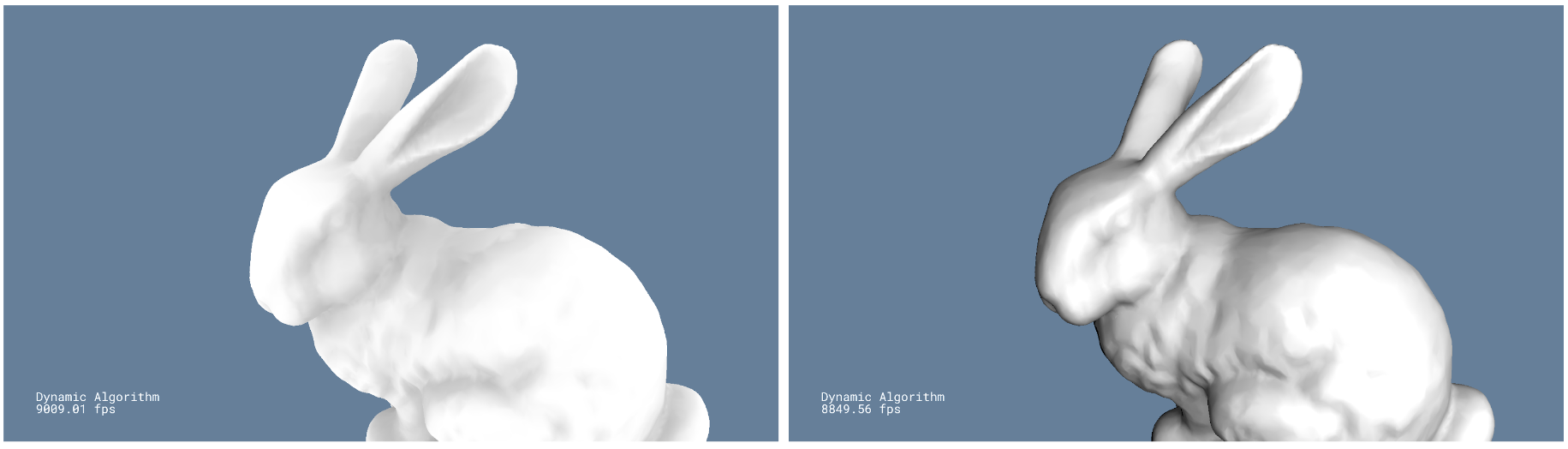
The left figure shows the result of ambient occlusion only. The lighting with bent normals is also applied in the right figure.

2. High Quality Ambient Occlusion [2]

Disks

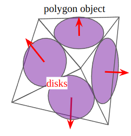
This algorithm converts polygon data from an object to disks, which are created per-face. Similar to dynamic ambient occlusion algorithm, each disk has its own centroid, normal, and area information. The centroid is the averaged position of vertices in a face. The normal can be calculated from the vertices using cross product. The Area can be also taken with the same way in dynamic ambient occlusion algorithm. So this algorithm does not require the additional search to find how many faces a vertex shares.

Occlusion Tree

After creating disks from all the vertices, a tree should be built. The structure of this tree is essentially same with the surface elements tree. The key point is still the same: for the efficient traversal, the next link of the last child of a node should point to the next of its parent. To separate these disks, however, texture coordinates is not necessary. Instead of that, the sorting by centroids towrads the dominant axis is used. So in this process all disks become leaf nodes, their parent nodes are created whose centroid/normal/area information are calculated from their children as processed in dynamic ambient occlusion algorithm. While the area of parent node is the sum of the areas of children, the centroid and normal of parent node is calculated differently. These can be done with the weighted sum because each child can produce a weight from its area and the total area, or the area of the parent node.

Shadow Approximation

The formula of shadow approximation [2] suggests actually comes from the form factor approximation in [1] as follows: $$\begin{aligned} \overbrace{\frac{A/\pi}{A/\pi + d^2}}^{\text{part D}} \cdot s(\cos \theta_E) \cdot s(\cos \theta_R) \end{aligned}$$

The part D looks similar to the part A, and I think that is because it is approximated based on solid angle. If the part A assumes that the spherical surface area approximate the area of the emitter, the spherical surface area does not need to be calculated at first. Instead of that, this area can be replaced by $A = \pi r^2$. That is, the solid angle can be approximated, not the spherical suface area, this time. $$\begin{aligned} \omega = \frac{A}{R^2} = \frac{\pi r^2}{R^2} \end{aligned}$$

In addition, the total angle is not necessarily $2\pi$ since the front facing of the receiver is the only interest, which means that the total angle is based on the hemisphere. Therefore, the occlusion ratio by the emitter is $$\begin{aligned} \frac{\omega}{\pi} = \frac{r^2}{R^2} = \frac{A/\pi}{A/\pi + d^2} = \text{ part D.} \end{aligned}$$

Robust Solution

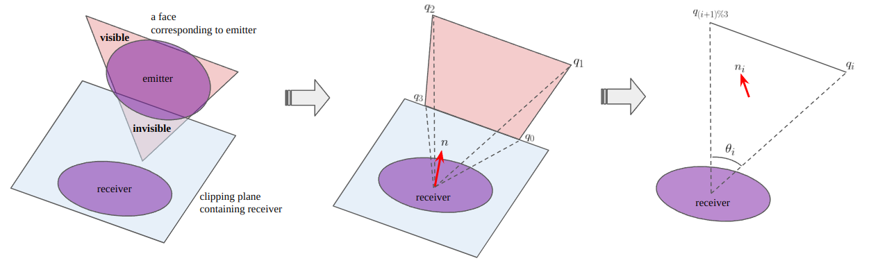
The specialty of this high quality ambient occlusion algorithm is its robustness. This algorithm calculates disk-to-disk ambient occlusion for a few passes, but in the last pass this computes fragment-to-disk occlusion more accurately. For a few passes, the shadow values are accumulated with the shdow approximation formula. In the last pass, the occlusion is calcualted with the form factor formula only for the visible portion of the face corresponding to the emitter by clipping with the plane containing the receiver as shown in the above figure. The clipped triangle face can have maximum four points. Let these points be $q_0, q_1, q_2$ and $q_3$. Given that the normal of the receiver, $n$, the form factor is $$\begin{aligned} \frac{1}{2\pi} \sum_{0 \leq i \leq 3} \theta_i \cdot \text{ dot}(n, n_i) \end{aligned}$$

where $\theta_i$ and $n_i$ are described in the above figure.

Modulation is applied as well. Other than the accessibility of the emitter element from the last pass as dynamic ambient occlusion algorithm, distance attenuation $a_D$ is also considered. The shadow value is modulated by being divided by $1 + a_D \cdot d$. Besides, triangle attenuation $a_T$ is introduced for the final pass. The shadow value should be multiplied by the previous accessibility $x$ to the power of $a_T$, that is $x^{a_T}$, then distance attenuation is applied. With low triangle attenuation, small features like creases and cracks are emphasized. With high triangle attenuation, the influence of far away (probably invisible) triangles is lessened.

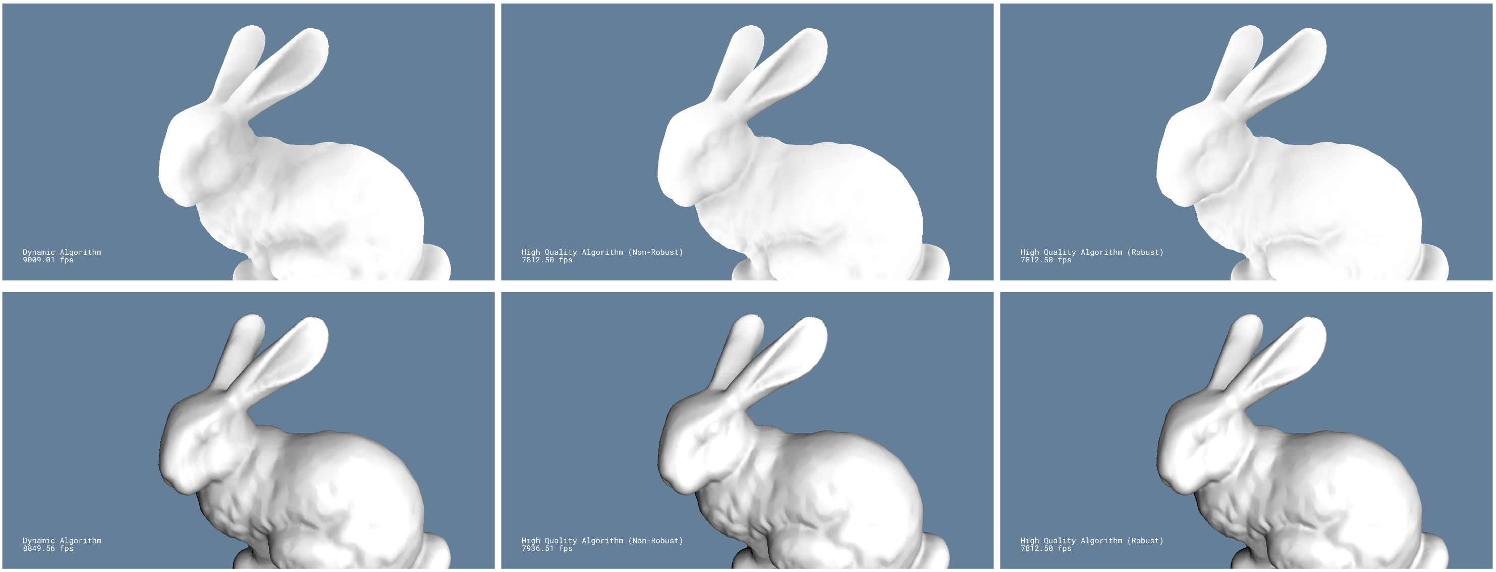
Result

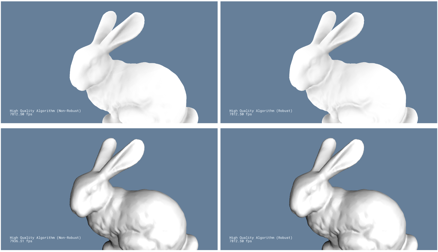
The top row figures show the result of ambient occlusion only. The lighting with bent normals is also applied in the bottom row figures. While the left column figures are rendered without the robust algorithm, the ones in the right column are done with the robust algorithm.

References

[1] Chapter 14. Dynamic Ambient Occlusion and Indirect Lighting

[2] Chapter 12. High-Quality Ambient Occlusion

[3] https://github.com/QianMo/GPU-Gems-Book-Source-Code/blob/master/GPU-Gems-2-CD-Content/Shading_Lighting_and_Shadows/Ch_14_Dynamic_Ambient_Occlusion_and_Indirect_Lighting/occlusion.cg

Code

https://github.com/emoy-kim/AmbientOcclusion