Quintic Equation
- Step 1. Find the upper and lower bounds of real roots
- Step 2. Find the extrema of
- Step 3. Select ranges containing a root
- Step 4. Ostrowski’s method
- References
Consider a quintic equation
Even though it is a well-known fact that there is no general solution in radicals to degree five or higher polynomial equations as proved by Abel-Ruffini theorem, it is possible to find approximately the roots of .
Step 1. Find the upper and lower bounds of real roots
First of all, determine the search range. With the geometrical properties of polynomial roots, there are some methods to get the bounds of real roots. Among them, an application of Cauchy’s bound can set an upper bound as follows.
For a lower bound, it suffices to apply this formula to and then multiply by the result.
Step 2. Find the extrema of
Next, the extrema should be obtained from the first derivative . This requires solving a quartic equation and this note explains how to do this. These extrema are used to set ranges to find each root. Note that any inflection point will not be counted because it cannot be an extremum since is polynomial.
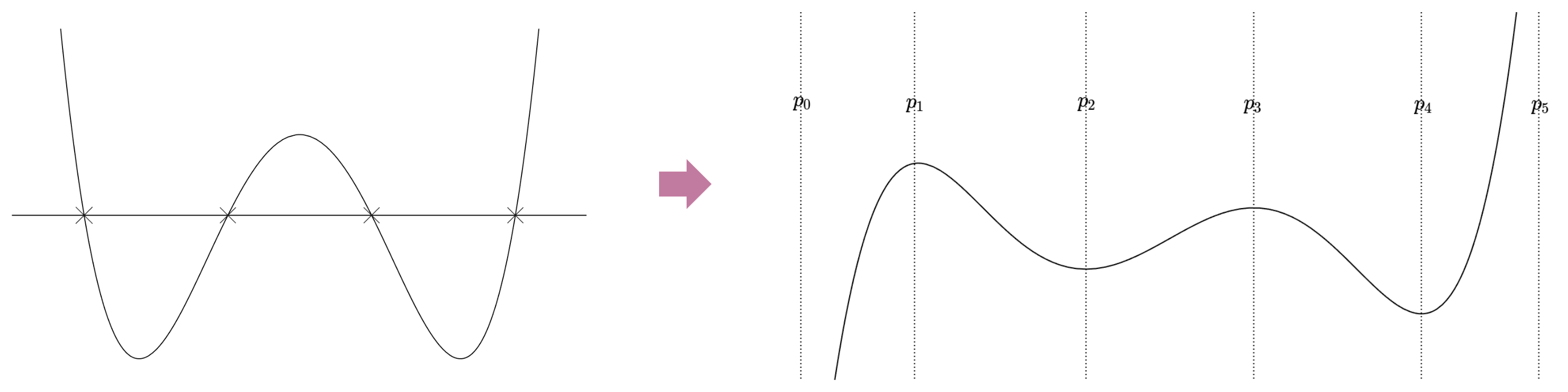
Step 3. Select ranges containing a root
This step aims to set ranges worthy to run an iterative method to find roots. The found extrema are used to set the initialization of an iterative method since a root is probably located between the adjacent extrema. For this, all the extrema must be sorted first including the upper and lower bounds. Given the number of extrema, let be the -th element in the sorted list. Note that is the lower bound and is the upper bound. is an extremum sorted in increasing order only when . The possible value of is always , , or .
Case 1.
Case 2.
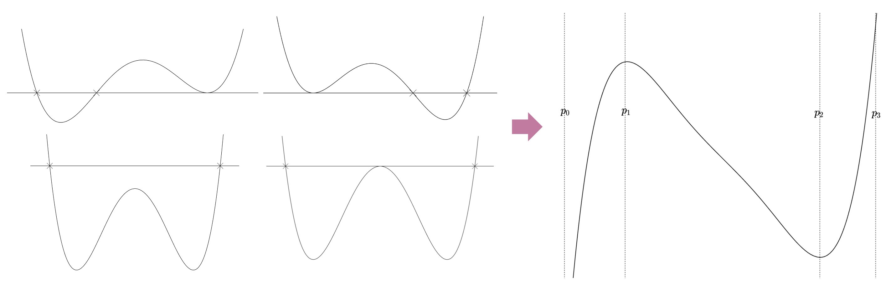
Case 3.
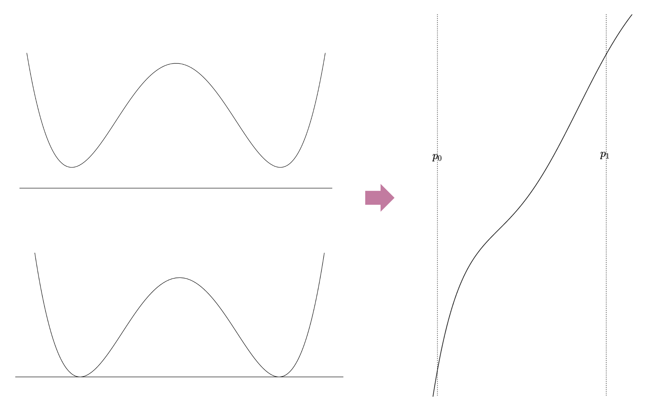
Then, which range should be selected? It depends that is increasing or decreasing in that range. But, in both cases, surely any root cannot be found if . As another corner case, means that or is the root. However, it is safe to assume that since this search is left-to-right and will double skip when happens as follows.
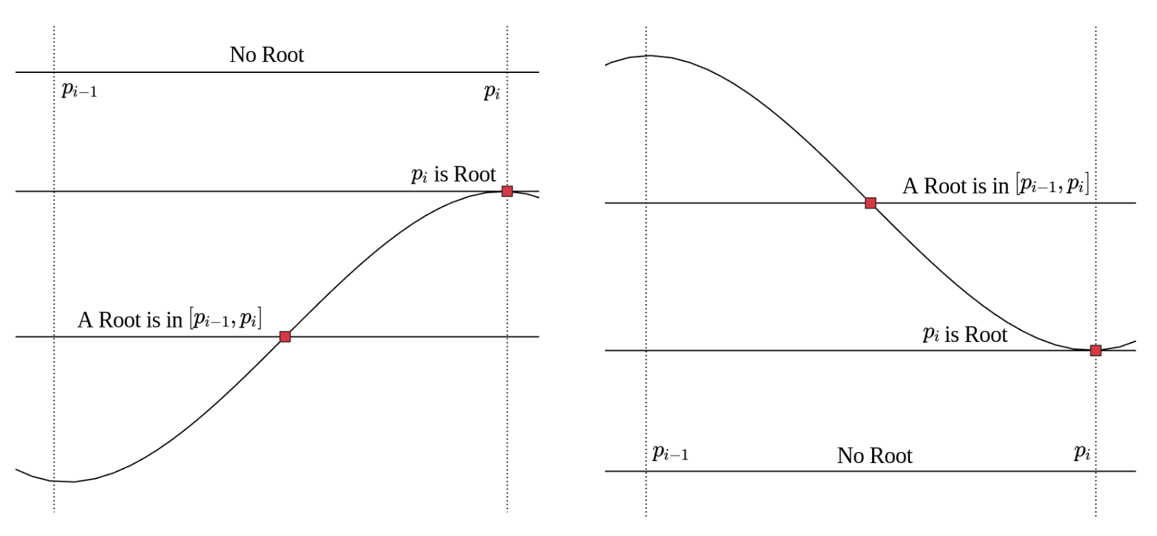
If is increasing in ,
- is the root when , and skip range because this range does not need to be searched.
- There is no root if , and skip range because this range does not need to be searched.
- There exists a root when .
If is decreasing in ,
- is the root when , and skip range because this range does not need to be searched.
- There is no root if , and skip range because this range does not need to be searched.
- There exists a root when .
Note that the case that is increasing above the -axis or is decreasing below the -axis is naturally skipped.
Step 4. Ostrowski’s method
After selecting ranges containing a root, the iterative method can be run in these ranges. Since the increasing or decreasing trend in each range is not changed, the initialization of the iterative method may be set as follows.
Newton’s method or Halley’s method might be used for this step, but Ostrowski’s two-point method yields a better efficiency index than both the Newton and the Halley methods since it reaches a fourth-order convergence rate. Ostrowski’s method can be derived from double Newton’s method, and its geometric approach looks like the below figure.
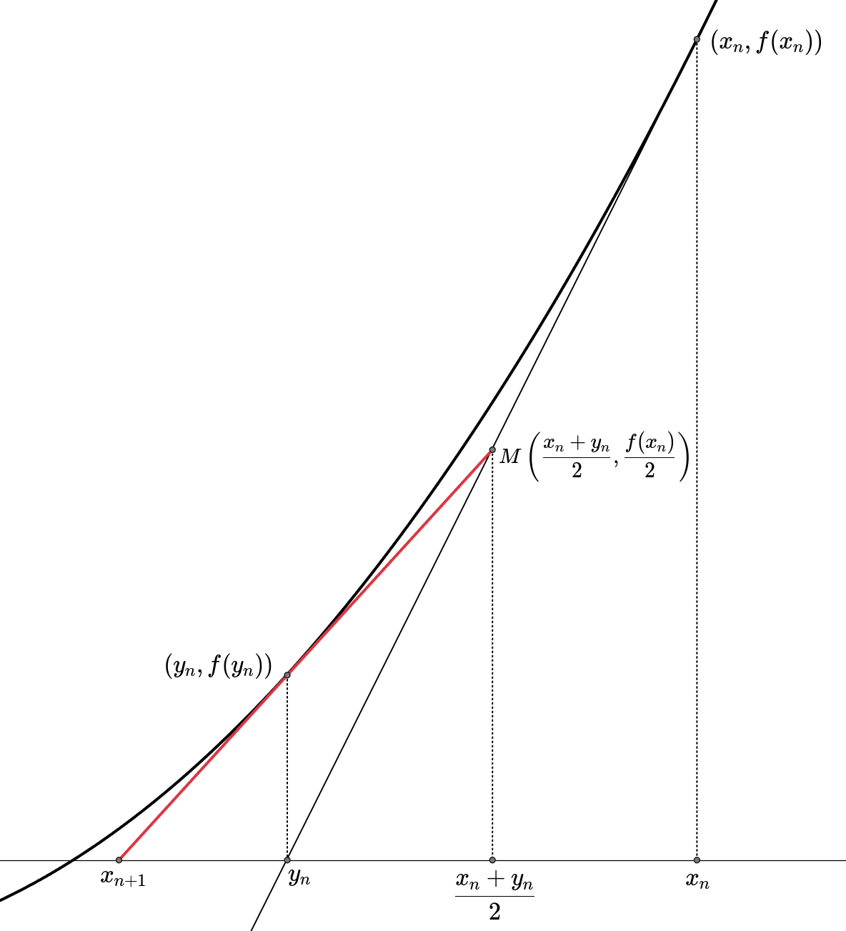
Let be the updated result of from the Newton’s method. Then,
Now, let be the midpoint of and . The intersection between the -axis and the line drawn through and is considered as the updated point, . From the similarity,
After arranging this equation and substituting by the form of ,
In conclusion, this method is divided into two steps.
It is worth noting that this method’s convergence order is reduced when encountering multiple roots. However, step 3 would already handle if the multiple roots exist because this case could be caught by testing . Also, it is guaranteed that each range has a root since its increasing or decreasing trend is consistent.
References
[1] Fast and Stable Polynomial Root Finders - Part Six
[2] Miodrag Petkovic, Beny Neta, Ljiljana Petkovic, and Jovana Dzunic. 2013. MULTIPOINT METHODS FOR SOLVING NONLINEAR EQUATIONS (1st. ed.). Academic Press, Inc., USA.