Some Facts about Eigenvalues

1. Localizing Eigenvalues

• It is useful when we want to know the rough location of eigenvalues of a matrix.
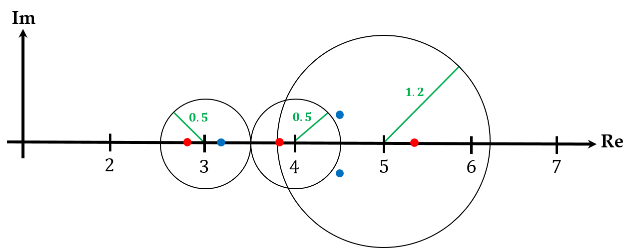
• Gershgorin’s Theorem says that all the eigenvalues of an $n \times n$ matrix $A$ is within $n$ disks. The $k$-th disk of these $n$ disks is centered at $a_{kk}$ and its radius is $\sum_{j \not = k} \vert a_{kj} \vert$ where $a_{ij}$ is $(i, j)$ element of $A$.
• Suppose that $x$ is the eigenvector of $A$ and $\lambda$ is the eigenvalue of $x$ such that $\left\| x \right\|_{\infty} = 1$. Then there exists $x_k = 1$ in $x$.

$$\begin{aligned} Ax = \lambda x &= \left(\begin{array}{ccccc} & & \vdots & & \\ a_{k1} & \cdots & a_{kk} & \cdots & a_{kn} \\ & & \vdots & & \end{array}\right) \left(\begin{array}{c} x_1 \\ \vdots \\ x_k \\ \vdots \\ x_n \end{array}\right) = \lambda \left(\begin{array}{c} x_1 \\ \vdots \\ x_k \\ \vdots \\ x_n \end{array}\right) \\ &\implies a_{k1}x_1 + \cdots + a_{kk}x_k + \cdots + a_{kn}x_n = \lambda x_k \\ &\implies (\lambda - a_{kk})x_k = \lambda - a_{kk} = \sum_{j \not = k} a_{kj}x_j \\ &\implies \vert \lambda - a_{kk} \vert = \left\vert \sum_{j \not = k} a_{kj} x_j \right\vert \le \sum_{j \not = k}\vert a_{kj} \vert \vert x_j \vert \le \sum_{j \not = k}\vert a_{kj} \vert = \text{radius} \end{aligned}$$

• For example, the eigenvalues of $A_1$ and $A_2$ are as follows:

$$\begin{aligned} A_1 = \left(\begin{array}{ccc} \color{blue}4.0 & -0.5 & 0.0 \\ 0.6 & \color{blue}5.0 & -0.6 \\ 0.0 & 0.5 & \color{blue}3.0 \end{array}\right), \quad A_2 = \left(\begin{array}{ccc} \color{red}4.0 & 0.5 & 0.0 \\ 0.6 & \color{red}5.0 & 0.6 \\ 0.0 & 0.5 & \color{red}3.0 \end{array}\right) \end{aligned}$$

$A_1$ and $A_2$ have the same diagonal elements and sum of absolute values in each row except the diagonal element, so their disks are the same. As above, the blue circles are the eigenvalues of $A_1$ and the red circles are those of $A_2$.

2. Sensitivity

• It is about the sensitivity of the eigenvectors and eigenvalues to small changes in an $n \times n$ matrix $A$.
• Suppose that an $n \times n$ matrix $X = (x_{(1)}, \cdots, x_{(n)})$ where $x_{(i)}$ is the eigenvector of $A$ and $n \times n$ diagonal matrix $D = diag(\lambda_1, \cdots, \lambda_n)$ where $\lambda_i$ is the eigenvalue corresponding to $x_{(i)}$. Then $AX = XD$.
• When all the eigenvectors of $A$ are nondefective, which means they are linearly independent, $X^{-1}AX = D$. After $A$ goes through some small changes, assume that $A$ turns into $A+E$ where $E$ denotes errors. Then $X^{-1}(A+I)X = X^{-1}AX + X^{-1}EX = D+F$. Since $A+E$ and $D+F$ are similar, they must have the same eigenvalues. Let $\mu$ be an eigenvalue of $A+E$, then for the eigenvector $v$ corresponding to $\mu$,

$$\begin{aligned} (D+F)v = \mu v \implies v = (\mu I - D)^{-1}Fv \end{aligned}$$

For this to be true, $(\mu I - D)$ should be nonsingular which happens when all its diagonal elements are not zero. It means that any elements of $D$ should not have $\mu$. Otherwise, $D$ has the eigenvalue $\mu$, so $F = 0$ and $E = 0$ which mean there are no errors. However, we consider $E \not = 0$, so $(\mu I - D)$ is nonsingular. Accordingly, $$\begin{aligned} \left\|v\right\|_2 \le \left\|(\mu I - D)^{-1}\right\|_2 \left\|F\right\|_2 \left\|v\right\|_2 \implies \left\|(\mu I - D)^{-1}\right\|_2 \le \left\|F\right\|_2 \end{aligned}$$

By definition, $\left\|(\mu I - D)^{-1}\right\|_2$ is the largest singular value. Therefore $\left\|(\mu I - D)^{-1}\right\|_2 = \frac{1}{\mu - \lambda_k}$ where $\lambda_k$ is the eigenvalue of $D$ closest to $\mu$. $$\begin{aligned} \left\|(\mu I - D)^{-1}\right\|_2 &= \vert \mu - \lambda_k \vert \le \left\|F\right\|_2 = \left\|X^{-1}EX\right\|_2 \\ &\le \left\|X^{-1}\right\|_2 \left\|E\right\|_2 \left\|X\right\|_2 = \text{condition number}(X)\left\|E\right\|_2 \end{aligned}$$

So, the effect from a small change of $A$ depends on the condition number of $X$, not the condition number of $A$.

• Another way to check the sensitivity of eigenvalues and eigenvectors including even when $A$ is defective is using right and left eigenvectors together. Let $x$ and $y$ be right and left eigenvectors, then there exist $\lambda$ and $\mu$ such that $Ax = \lambda x$ and $y^t A = \mu y^t$. It yields that $y^t Ax = \lambda y^t x = \mu y^t x$, so $\lambda = \mu$ or $y^t x = 0$. Assume that $y^t x \not = 0$. If $A$ has been changed by an error $E$ and $x$ and $\lambda$ are also changed, then

$$\begin{aligned} (A+E)(x + \Delta x) &= (\lambda + \Delta \lambda)(x + \Delta x) \\ Ax + Ex + A \Delta x + E \Delta x &= \lambda x + \Delta \lambda x + \lambda \Delta x + \Delta \lambda \Delta x \\ Ex + A \Delta x + E \Delta x &= \Delta \lambda x + \lambda \Delta x + \Delta \lambda \Delta x \\ Ex + A \Delta x &\approx \Delta \lambda x + \lambda \Delta x \end{aligned}$$

because $E \Delta x$ and $\Delta \lambda \Delta x$ are small enough and negligible. Since $\lambda = \mu$, we can add $y$ as follows: $$\begin{aligned} y^t Ex + y^t A \Delta x &\approx \Delta \lambda y^t x + \lambda y^t \Delta x \\ y^t Ex &\approx \Delta \lambda y^t x \\ \Delta \lambda &\approx \frac{y^t Ex}{y^t x} \\ \vert \Delta \lambda \vert &\lessapprox \frac{\left\| y \right\|_2 \left\| x \right\|_2}{\left\| y^t x \right\|_2} \left\| E \right\|_2 = \frac{1}{cos\theta} \left\| E \right\|_2 \end{aligned}$$

where $\theta$ is the angle between $x$ and $y$. So, it is sensitive as $\theta$ increases.

• For example,

$$\begin{aligned} A &= \left(\begin{array}{ccc} -149 & -50 & -154 \\ 537 & 180 & 546 \\ -27 & -9 & -25 \end{array}\right) \\ \\ \text{eigenvalues: } \lambda_1 &= 1, \; \lambda_2 = 2, \; \lambda_3 = 3 \\ \\ \text{normalized right eigenvectors: } X &= \left(\begin{array}{ccc} x_{(1)} & x_{(2)} & x_{(3)} \end{array}\right) = \left(\begin{array}{ccc} 0.316 & 0.404 & 0.139 \\ -0.949 & -0.909 & -0.974 \\ 0.000 & -0.101 & 0.179 \end{array}\right) \\ \\ \text{normalized left eigenvectors: } Y &= \left(\begin{array}{ccc} y_{(1)} & y_{(2)} & y_{(3)} \end{array}\right) = \left(\begin{array}{ccc} 0.681 & -0.676 & -0.688 \\ 0.225 & -0.225 & -0.229 \\ 0.697 & -0.701 & -0.688 \end{array}\right) \end{aligned}$$

First, the condition number of $X$ is $1289$, so the eigenvalues of $A$ are sensitive. Second, $y^t_{(1)} x_{(1)} = 0.0017$, $y^t_{(2)} x_{(2)} = 0.0025$, and $y^t_{(3)} x_{(3)} = 0.0046$, so the angles between $x_{(i)}$ and $y_{(i)}$ are large. Therefore, it is expected that $A$ is sensitive to small changes. The following are eigenvalues changed from tiny changes of $A$. $$\begin{aligned} A + E &= \left(\begin{array}{ccc} -149 & -50 & -154 \\ 537 & \color{red}180.01 & 546 \\ -27 & -9 & -25 \end{array}\right) \implies \begin{cases} \lambda_1 = 0.207 \\ \lambda_2 = 2.301 \\ \lambda_3 = 3.502 \end{cases} \\ \\ A + E &= \left(\begin{array}{ccc} -149 & -50 & -154 \\ 537 & \color{red}179.99 & 546 \\ -27 & -9 & -25 \end{array}\right) \implies \begin{cases} \lambda_1 = 1.664 + 1.054i \\ \lambda_2 = 1.664 - 1.054i \\ \lambda_3 = 2.662 \end{cases} \end{aligned}$$

It shows the large changes of eigenvalues about the small changes of $A$.

3. Properties

• Suppose that $x$ is the eigenvector of an $n \times n$ matrix $A$ and $\lambda$ is the eigenvalue corresponding to $x$.
• $A$ has the eigenvalue which is zero

$\iff$ There exists $x \not = 0$ such that $Ax = 0$

$\iff$ $\dim Ker A > 0$

$\iff$ $A$ is singular

• For $\alpha \not = 0 \in \R$, $\alpha x$ is also the eigenvector of $A$.
• $x$ is the eigenvector of $\alpha A$ for $\alpha \in \R$, and its eigenvalue is $\alpha \lambda$.
• $x$ is the eigenvector of $A + \alpha I$ for $\alpha \in \R$, and its eigenvalue is $\lambda + \alpha$.
• For $k \in \N$, $x$ is the eigenvector of $A^k$, and its eigenvalue is $\lambda^k$.
• If $A$ is invertible, $x$ is the eigenvector of $A^{-1}$, and its eigenvalue is $\frac{1}{\lambda}$.
• For a diagonal matrix $D = diag(a_1, \cdots, a_n)$, its eigenvalues are $a_1, \cdots, a_n$ and its eigenvectors are $e_1, \cdots, e_n$ where all components of a standard basis vector $e_i \in \R^n$ are $0$ except the $i$-th element which is $1$.
• For upper or lower triangular matrices, the eigenvalues are their diagonal elements.
• For an $n \times n$ nonsingular matrix $S$, $S^{-1}x$ is the eigenvector of $S^{-1}AS$ and the eigenvalue corresponding to $S^{-1}x$ is $\lambda$. Eigenvalues are not changed by similar transformations.
• $\det A = \lambda_1 \cdots \lambda_n$.
• For $k \le n$, if eigenvalues $\lambda_1, \cdots, \lambda_k$ are distint, the eigenvectors $x_{(1)}, \cdots, x_{(n)}$ corresponding to them are linearly independent.
• If all the eigenvalues are distint, all the eigenvectors are linearly independent, so $X = (x_{(1)}, \cdots, x_{(n)})$ is nonsingular and diagonalizable as $X^{-1}AX = diag(\lambda_1, \cdots, \lambda_n)$. However, although $X$ is diagonalizable, its all eigenvalues may not be distint such $A = I$. Moreover, although the eigenvalues of $A$ are not unique, $A$ may be diagonalizable. For example,

$$\begin{aligned} A + E &= \left(\begin{array}{ccc} 3 & -1 & 1 \\ 0 & 2 & 1 \\ 0 & 0 & 3 \end{array}\right) \implies \begin{cases} \lambda_1 = 2 \\ \lambda_2 = 3 \\ \lambda_3 = 3 \end{cases} \\ &\implies X = \left(\begin{array}{ccc} 1 & 1 & 0 \\ 1 & 0 & 1 \\ 0 & 0 & 1 \end{array}\right) \text{: nonsingular} \end{aligned}$$

• Singular values of $A$ are the nonnegative square roots of eigenvalues of $A^t A$.

References

[1] Michael T. Heath, Scientific Computing: An Introductory Survey. 2nd Edition, McGraw-Hill Higher Education.

[2] Hiraoka Kazuyuki, Hori Gen, Programming No Tame No Senkei Daisu, Ohmsha.