Matting is a technique that extracts the foreground from an image.
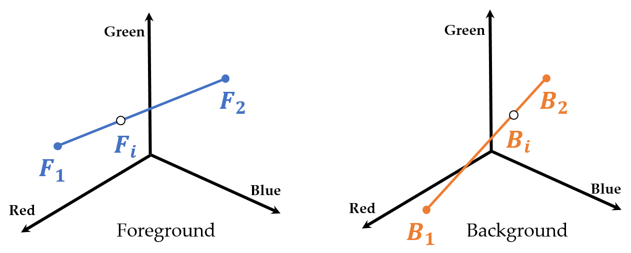
Matting needs an assumption that for a small window w of an image, its foreground pixels are colinear, so are its background pixels.
More specifically, for a pixel i∈w, there exists βi, γi, F1, F2, B1, and B2 such that Fi=βiF1+(1−βi)F2 and Bi=γiB1+(1−γi)B2 where Fi is the foreground component of the pixel i and Bi is the background component of it.
Moreover, the intensity Ii of the pixel i consists of Fi and Bi such that Ii=αiFi+(1−αi)Bi for some αi.
So αi=r1tIi−r1tB2. It implies that αi and Ii are in a linear relationship for w. It means that for every window Ii and αi are in an affine relationship.
2. Matting Laplaciain
For the affinity of Ii and αi, αi≈aIi+b for some a and b. Now consider the cost function J(α,a,b).
j=1∑Ni∈wj∑(αij−(ajIij+bj))2+ϵ∥aj∥22
where N is the number of windows in an image which is the same as the number of pixels in an image because the windows are created for each pixel. As the regularization term of this cost function, ϵ∥aj∥22, is minimized, aj goes to zero, and it causes ai≈bj. Here assume that Ii is a scalar for simplicity, but it can be also extended to a three-dimensional vector.
Let Gj(GjtGj)−1Gjt=X, then Xt=Gj(GjtGj)−1Gjt=X, so X is symmetric. Moreover, XXt=XX=Gj(GjtGj)−1GjtGj(GjtGj)−1Gjt=Gj(GjtGj)−1Gjt=X. It implies that J(α)=j=1∑N∥Xαj−αj∥2=j=1∑N∥(X−I)αj∥2=j=1∑Nαjt(X−I)t(X−I)αj=j=1∑Nαjt(Xt−I)(X−I)αj=j=1∑Nαjt(XtX−X−Xt+I)αj=j=1∑Nαjt(X−X−Xt+I)αj=j=1∑Nαjt(I−X)αj=j=1∑Nαjt(I−Gj(GjtGj)−1Gjt)αj=j=1∑NαjtGjαj
Besides, GjtGj, (GjtGj)−1, (GjtGj)−1Gjt, and Gj(GjtGj)−1Gjt are as follows:
where u, v∈[1,W] are integers. From equations as above, (Gjuv) which means the (u,v) element of Gj is (Gj)uv=(I−Gj(GjtGj)−1Gjt)uv=δuv−Wσ2+ϵ1(IuIv−Iuμ+σ2+μ2−Ivμ+Wϵ)=δuv−Wσ2+ϵ1(σ2+Wϵ+(Iu−μ)(Iv−μ))=δuv−W1(1+σ2+Wϵ1(Iu−μ)(Iv−μ))
where \delta_{uv} is the Kronecker delta which means that 1 if u=v and 0 otherwise.
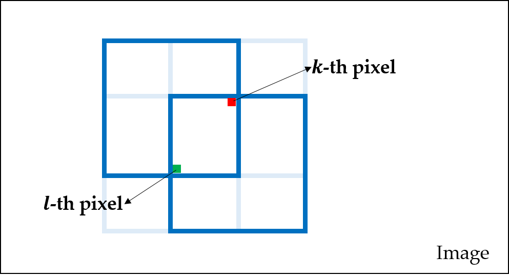
Let the top-left W×W submatrix of Gj be [Gj]. Now, J(α) can be represented as the form mtLm where L is the Matting Laplacian. Particularly, m is an N×1 matte vector where mk is the matte of the k-th pixel. Therefore, there exist multiple i and j pairs such that αij=mk.
Lkl appears in only mkLklml part. Therefore, Lkl is the sum of the coefficients of αi1j1αi2j2 pairs which are equivalent to mkml in ∑j=1NαjtGjαj.
In other words, for the window-set wkl that includes the k-th and l-th pixels together in an image, Lkl can be figured out from this by calculating ∑w∈wklαwtGwαw. This is because there exists the set Θ={(pw,qw)∣pw=mk,qw=ml,pw,qw∈αw and w∈wkl}. Therefore, Lkl is as follows: Lkl=w∈wkl∑(Gw)pwqw=w∈wkl∑δpwqw−Wpwqw1(1+σw2+Wϵ1(Ipw−μw)(Iqw−μw))
L is symmetric since Lkl=Llk.
Finally, J=mtLm, so it can be solved by solving Lm=0 because ∂m∂J=2mtL=0.
3. Adding Constraint
Any constant m is in nullspace of L. Consider cL(1,⋯,1)t for c∈R. Then its i-th row element is ∑j=1NLij. For the window-set wii that includes the i-th pixel, let pw=mi, w∈wii. Then,
So user scribbles are required which denote some of foreground and background pixels in an image. Let U be a N×1 vector whose i-th element is 1 if it is the known foreground pixel or 0 otherwise. In addition, let F={f∣Uf=1}.
J=minmtLm+λf∈F∑(mf−1)2=minmtLm+λ(m−U)tD(m−U)
where D is an N×N diagonal matrix which Dii=1 if Ui=1 or 0 otherwise.
Therefore, the solution can be from the linear system (L+λD)m=λU where λ is a large number, for example, 100.
4. The eigenvectors of L
Without user scribbles, the solution of J=mtLm is that of Lm=0.
Consider Lv=λv where v is the eigenvector of L and λ is the eigenvalue of v. If we choose λ closing to 0, then Lv=λv≈0=Lm.
This eigenvector v looks like a grayscale image.
Let the set Φ={v∣Lv=λv,λ≈0}. Then for s=∣Φ∣, Lv1+⋯+Lvs=L(v1+⋯+vs)≈0. It means that any combination of elements in Φ can be a candidate of m. More formally, there exist some constants such that m≈∑i=1scivi and ∑i=1sci=1 for c∈R. However, it is more realistic that we define an N×1 vector β such that m≈∑i=1sβivi and ∑i=1sβi,j=1 where βi,j denotes the j-th element of βi for 1≤j≤N.
Meanwhile, it is likely that most elements of m are 0 or 1 in the ground truth of m. This is because most mi is in range (0,1) only when the i-th pixel is in the boundary of the foreground. So, it is reasonable that if m is well estimated, most elements of m are 0 or 1.
Therefore, J can be reformed as follows:
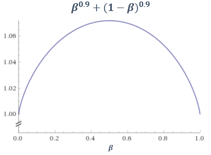
J=mini=1∑sj=1∑N∣βi,j∣ρ+∣1−βi,j∣ρ
Each βi is forced to be distributed to 0 or 1 when it is minimized. This cost function produces a good solution even when user scribbles are not given.
Reference
[1] Richard J. Radke, (2012) Computer Vision for Visual Effects, Cambridge University Press, Cambridge.
Keep going!Keep going ×2!Give me more!Thank you, thank youFar too kind!Never gonna give me up?Never gonna let me down?Turn around and desert me!You're an addict!Son of a clapper!No wayGo back to work!This is getting out of handUnbelievablePREPOSTEROUSI N S A N I T YFEED ME A STRAY CAT