Things about Algorithm Concepts

• 1. For an arbitrary sequence $\, a_{nn}$ of certain elements numbered by two indices, the following holds.
• 2. Approximation of Harmonic Number
• 3. $n!$ is divisible by $\, p^\mu$ where $\, n$ is a natural number and $\, p$ is a prime number, and $\, \mu$ is defined by
• 4. Chebyshev’s Inequality
• 5. The mean and variance are easily from the generating function.
• 6. The mean and variance of two generating functions are summations of each one of them.
• 7. When running into the $0/0$-form, consider Taylor’s theorem as a workaround.
• 8. Any forest to a binary tree
• 9. Huffman algorithm to find a tree with minimum weighted path length
• Reference

1. For an arbitrary sequence $\, a_{nn}$ of certain elements numbered by two indices, the following holds.

$$\begin{aligned} \sum_{i = 1}^{n} \sum_{j = 1}^{i} a_{ij} = \sum_{j = 1}^{n} \sum_{i = j}^{n} a_{ij} \end{aligned}$$

This arises from the following facts. This logic process is useful and can be applied to other similar problems. $$\begin{aligned} &1 \leq i \leq n \text{ and } 1 \leq j \leq i \\ \Longleftrightarrow \; &1 \leq j \leq i \leq n \\ \Longleftrightarrow \; &1 \leq j \leq n \text{ and } j \leq i \leq n \end{aligned}$$

2. Approximation of Harmonic Number

Harmonic number $H_n$ is defined by $$\begin{aligned} H_n = 1 + \frac{1}{2} + \frac{1}{3} + \cdots + \frac{1}{n} = \sum_{k = 1}^n \frac{1}{k}, \quad n \geq 0 \end{aligned}$$

The approximate size of this harmonic number is a well-known quantity as follows. $$\begin{aligned} H_n = \ln n + \gamma + \frac{1}{2n} - \frac{1}{12n^2} + \frac{1}{120n^4} - \epsilon, \quad 0 < \epsilon < \frac{1}{252n^6} \end{aligned}$$

where $\gamma = 0.5772156649\dots$ is Euler’s constant. Thus $H_n$ is reasonably close to the natural logarithm of $n$.

3. $n!$ is divisible by $\, p^\mu$ where $\, n$ is a natural number and $\, p$ is a prime number, and $\, \mu$ is defined by

$$\begin{aligned} \mu = \sum_{k > 0} \left \lfloor \frac{n}{p^k} \right \rfloor \end{aligned}$$

That is, $n!$ is divided by $p$ $\mu$ times. In other words, $\mu$ can be summed from the number of natural numbers having $p$-factor and the number of ones having $p^2$-factor and so on. For example, when $n = 1000$ and $p = 3$, $$\begin{aligned} \mu &= \left \lfloor \frac{1000}{3} \right \rfloor + \left \lfloor \frac{1000}{9} \right \rfloor + \left \lfloor \frac{1000}{27} \right \rfloor + \left \lfloor \frac{1000}{81} \right \rfloor + \left \lfloor \frac{1000}{243} \right \rfloor + \left \lfloor \frac{1000}{729} \right \rfloor + 0 + \cdots \\\\ &= 333 + 111 + 37 + 12 + 4 + 1 = 498 \end{aligned}$$

It means that $1000!$ is divisible by $3^{498}$ and is not by $3^{499}$. $\lfloor n / p^{k + 1} \rfloor = \lfloor \lfloor n / p^k \rfloor / p \rfloor$ is useful for more simple calculation. With a similar logic to this note, this can be proved as follows. $$\begin{aligned} &\quad m = \left \lfloor \frac{n}{p^{k + 1}} \right \rfloor \Longleftrightarrow m \leq \frac{n}{p^{k + 1}} < m + 1 \Longleftrightarrow mp \leq \frac{n}{p^{k}} < (m + 1)p \Longleftrightarrow \\\\ &mp \leq \left \lfloor \frac{n}{p^k} \right \rfloor < (m + 1)p \Longleftrightarrow m \leq \left \lfloor \frac{n}{p^k} \right \rfloor / p < m + 1 \Longleftrightarrow \left \lfloor \left \lfloor \frac{n}{p^k} \right \rfloor / p \right \rfloor = m \end{aligned}$$

So, the $k$-th step can be used for the $(k + 1)$-th step.

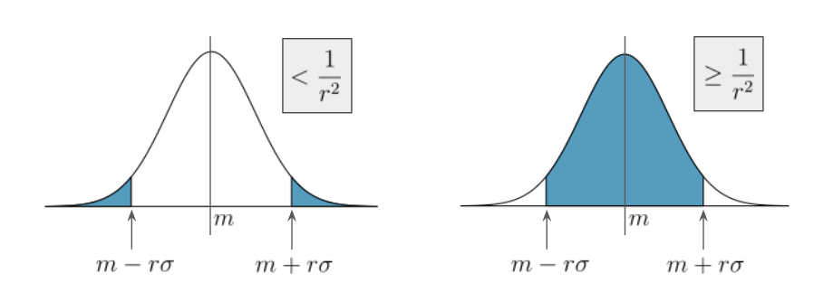
4. Chebyshev’s Inequality

For data $X$, let $m$ be the mean of $X$ and $V$ be the variance, then standard deviation $\sigma = \sqrt{V}$. $\sigma$ is important from the fact that the probability of $\vert x_i - m \vert > r \sigma$ is $< 1/r^2$ for any real number $r \geq 1$ and $x_i \in X$. Let this probability be $p$ and $p_i = P[X = i]$.

If $p > 0$, $$\begin{aligned} V &= \sum_{i} (x_i - m)^2 p_i = \sum_{\vert x_i - m \vert > r \sigma} (x_i - m)^2 p_i + \sum_{\vert x_i - m \vert \leq r \sigma} (x_i - m)^2 p_i \\\\ &> \sum_{\vert x_i - m \vert > r \sigma} (r \sigma)^2 p_i + 0 = (r \sigma)^2 \sum_{\vert x_i - m \vert > r \sigma} p_i = (r \sigma)^2 p = pr^2 V \\\\ \Longrightarrow \quad &pr^2 V < V \Longrightarrow \; p < \frac{1}{r^2} \end{aligned}$$

5. The mean and variance are easily from the generating function.

Generating function $G$ can be used whenever to obtain information about a sequence of numbers $a_n$. By obtaining information from $G$, information from $a_n$ can be obtained. $$\begin{aligned} G(z) = a_0 + a_1 z + a_2 z^2 + \cdots = \sum_{n \geq 0} z^n \end{aligned}$$

Consider the probabilities $p_k = P[X = k]$ as a sequence and generating function $G$ of them. Then, the mean $m$ and variance $V$ of $G$ can be defined as follows. $$\begin{aligned} G(z) = p_0 &+ p_1 z + p_2 z^2 + \cdots, \\\\ m = \sum_{k}k p_k, &\qquad V = \sum_{k}k^2 p_k - m^2 \end{aligned}$$

Note that $G(1) = p_0 + p_1 + p_2 + \cdots = 1$. Considering $G'(z)$, $m$ can be represented as $$\begin{aligned} G'(z) &= p_1 + 2 p_2 z + \cdots = \sum_{k} k p_k z^{k - 1}, \\\\ \Longrightarrow \quad & m = \sum_{k}k p_k = G'(1) \end{aligned}$$

Similarily, calculating $G''(z)$, $$\begin{aligned} G''(z) &= \sum_{k} k (k - 1) p_k z^{k - 2} = \sum_{k} (k^2 - k) p_k z^{k - 2}, \\\\ \sum_{k}k^2 p_k &= \sum_{k} (k^2 - k) p_k + \sum_{k} k p_k = G''(1) + G'(1), \\\\ \Longrightarrow \quad V &= \sum_{k}k^2 p_k - m^2 = G''(1) + G'(1) - G'(1)^2 \end{aligned}$$

6. The mean and variance of two generating functions are summations of each one of them.

Assume that $G$ and $H$ are generating functions for some probabilities, which means that $G(1) = H(1) = 1$. Let $m(X)$ and $V(X)$ be the mean and variance of probabilities represented by a generating function $X$. Then, the following holds. $$\begin{aligned} m(GH) = m(G) + m(H), \qquad V(GH) = V(G) + V(H) \end{aligned}$$

7. When running into the $0/0$-form, consider Taylor’s theorem as a workaround.

Consider a uniform distribution whose probability is $1/n$ of obtaining the values $1$, $2$, $\cdots$, $n$. The generating function of this is $$\begin{aligned} G(z) &= \frac{1}{n} z + \frac{1}{n} z^2 + \cdots + \frac{1}{n} z^n = \frac{1}{n} \frac{z^{n + 1} - z}{z - 1}, \\\\ G(1) &= \frac{1}{n} + \cdots + \frac{1}{n} = \frac{n}{n} = 1, \\\\ G'(z) &= \frac{nz^{n + 1} - (n + 1)z^n + 1}{n(z - 1)^2}, \\\\ G''(z) &= \frac{n(n - 1)z^{n + 1} - 2(n + 1)(n - 1)z^n + n(n + 1)z^{n - 1} - 2}{n(z - 1)^3} \end{aligned}$$

For finding the mean and variance, $G'(1)$ and $G''(1)$ are required but this makes the equations $0/0$ when $z = 1$. There exists a workaround. By Taylor’s theorem, $$\begin{aligned} G(1 + z) = G(1) + G'(1)z + \frac{G''(1)}{2!} z^2 + \cdots = 1 + G'(1)z + \frac{G''(1)}{2!} z^2 + \cdots \end{aligned}$$

Replacing $z$ by $z + 1$ in the original $G$ function and connecting this Taylor’s series, $$\begin{aligned} G(1 + z) = \frac{1}{n} \frac{(1 + z)^{n + 1} - 1 - z}{z} = 1 + G'(1)z + \frac{G''(1)}{2!} z^2 + \cdots \end{aligned}$$

Since the coefficient of $z$ is related to the coefficient of $z^2$ in $(1 + z)^{n + 1}$ and the coefficient of $z^2$ is related to the coefficient of $z^3$ in $(1 + z)^{n + 1}$, $$\begin{aligned} G'(1) &= \frac{1}{n} \left(\begin{array}{c} n + 1 \\ 2 \end{array}\right) = \frac{1}{n} \frac{(n + 1)!}{(n - 1)!\,2!} = \frac{1}{n} \frac{(n + 1)n}{2} = \frac{n + 1}{2} \\\\ \frac{G''(1)}{2!} &= \frac{1}{n} \left(\begin{array}{c} n + 1 \\ 3 \end{array}\right) = \frac{1}{n} \frac{(n + 1)!}{(n - 2)!\,3!} = \frac{1}{n} \frac{(n + 1)n(n - 1)}{6} = \frac{(n + 1)(n - 1)}{6} \end{aligned}$$

Therefore, the mean $m$ and variance $V$ are as follows. $$\begin{aligned} m &= G'(1) = \frac{n + 1}{2}, \\\\ V &= G''(1) + G'(1) - G'(1)^2 = \frac{(n + 1)(n - 1)}{3} + \frac{n + 1}{2} - \frac{(n + 1)^2}{4} \\\\ &= (n + 1)\left( \frac{n - 1}{3} + \frac{1}{2} - \frac{n + 1}{4} \right) = (n + 1)\frac{n - 1}{12} \end{aligned}$$

This is unstable situation. Generally, a distribution is called stable when the standard deviation is proportional to $\sqrt{n}$ and the difference between maximum and minimum is proportional to $n$.

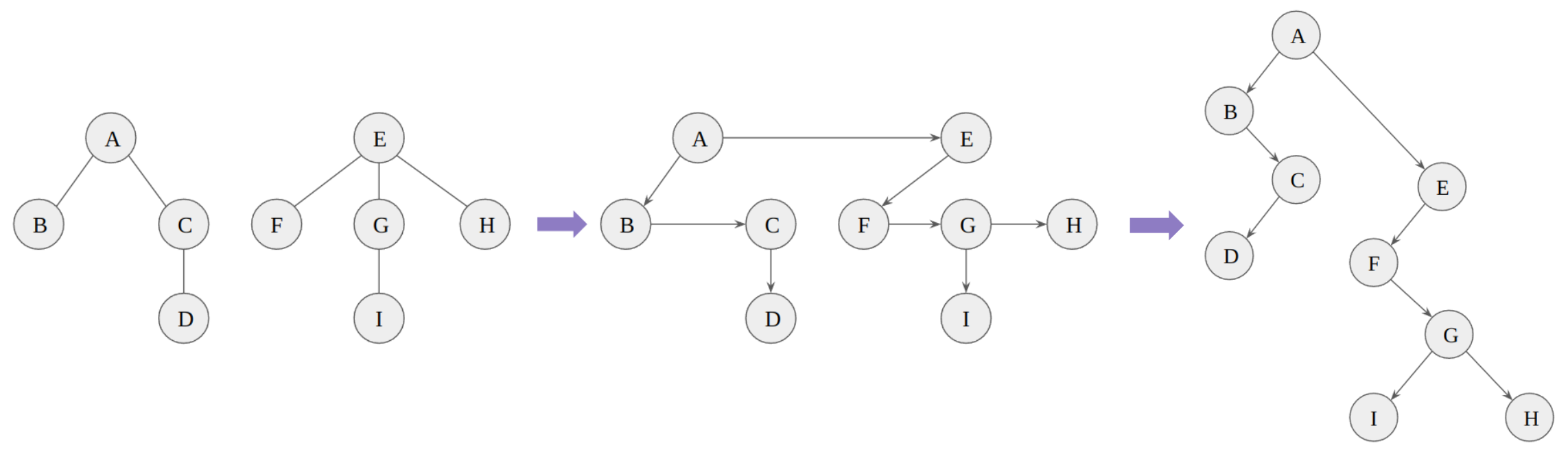
8. Any forest to a binary tree

There is a natural way to represent any forest as a binary tree.

1. Linking together the children of each family
2. Removing vertical links except from a parent to a first child

The final binary tree can be obtained after rotating the resulting tree. Note that any binary tree can be transformed into a unique forest by reversing the process.

9. Huffman algorithm to find a tree with minimum weighted path length

Given $m$ weights $w_1$, $w_2$, $\cdots$, $w_m$ that are all real numbers, the problem is to find a binary tree and to associate the weights with its nodes in such a way that the sum $\sum w_j l_j$ is minimized, where $l_j$ is the length of path from the root. The sum $\sum w_j l_j$ is also called weighted path lengths. Huffman algorithm is an elegant algorithm for this problem. First find the two $w$’s of lowest value, say $w_1$ and $w_2$. Then solve the problem for $m - 1$ weights $w_1 + w_2$, $w_3$, $\cdots$, $w_m$. Every time this construction combines two weights, they are at least as big as the weights previously combined, if the given $w_i$ were nonnegative. This means that there is a way to find Huffman’s tree, proveided that the given wieghts have been sorted into nondecreasing order. Using two queues, one containing the original wegiths and the other containing the combined wegiths, at each step the smallest unused weight will appear at the front of one of the queues. That is, there is no need to search for it. In general, there are many trees that minimize $\sum w_j l_j$. Furthermore, Huffman’s algorithm can be generalized to $t$-ary trees as well as binary trees.

Reference

[1] Donald E. Knuth, The Art of Computer Programming, Volume 1: Fundamental Algorithms