Green's Theorem

• Definition
• Line Integral
• Vector Field
• Discontinuous Integrand
• Application

Definition

This theorem implies that line integrals can be converted to surface integrals and vice versa. So, when a line integral is hard to calculate, the conversion to the surface integral may be considered. Let $C$ be a simple closed curve in $xy$-plane, and let $R$ be the region bounded by $C$. If $F_1$ and $F_2$ are functions of $(x, y)$ defined on an open region containing $R$ and have continuous partial derivatives, then $$\begin{aligned} \oint_D F_1 dx + F_2 dy &= \iint_R \left( \cfrac{\partial F_2}{\partial x} - \cfrac{\partial F_1}{\partial y} \right) dy dx \\ \text{line integral} &\iff \text{surface integral} \end{aligned}$$

Here, given a curve $C: [a, b] \in \mathbb{R}^2$, “$C$ is simple” means that $C(t_0) \ne C(t_1)$ for $a \leq t_0 < t_1 < b$, and “$C$ is closed” means that the starting point $C(a)$ and the end point $C(b)$ are the same. Accordingly, Green’s theorem implies that the line integral of a vector-valued function $\vec{F}(F_1, F_2)$ is the same as the area surrounded by that line, which means here that curve.

Line Integral

While a definite integral calculates along a fixed $x$-axis or $y$-axis, a line integral does along an arbitrary curve which is the more generalized version. Let the parametric curve $C$ of the length $s$ be on $xy$-plane. Then, $s$ can be viewed as the integral of $ds$ in $C$, and $ds$ is approximately a line segment. $$\begin{aligned} ds = \sqrt{(dx)^2 + (dy)^2} \implies s = \int_C ds = \int_a^b \sqrt{\left( \cfrac{d x}{d t} \right)^2 + \left( \cfrac{d y}{d t} \right)^2} dt \end{aligned}$$

Therefore, if a function $z = f(x, y)$ is integrated along $C$, $$\begin{aligned} \int_C f(x, y) ds = \int_a^b f(x(t), y(t)) \sqrt{\left( \cfrac{d x}{d t} \right)^2 + \left( \cfrac{d y}{d t} \right)^2} dt \end{aligned}$$

Note that when $f(x,y)=1$, this integral is $s$ since this integral becomes the area of a rectangle whose width is $s$ and height is $1$. Also, this concept can be similarly extended to $n$-dimension.

Vector Field

A line integral can be also done in a vector field. A vector field is an assignment of a vector to each point in a space. When a vector-valued function $\vec{F}(x, y, z)$ is integrated along a curve $C$, this integration represents the work of $\vec{F}$ done by a force moving along the curve path. If the curve $C$ is given as $X(t) = (x(t), y(t), z(t))$, the line integral of $\vec{F}$ is $$\begin{aligned} \int_C \vec{F}(X(t)) \cdot \left( \cfrac{dx}{dt}, \cfrac{dy}{dt}, \cfrac{dz}{dt} \right) dt \end{aligned}$$

This can be written more simply as $\displaystyle \int_C \vec{F} \cdot d\vec{s}$.

Discontinuous Integrand

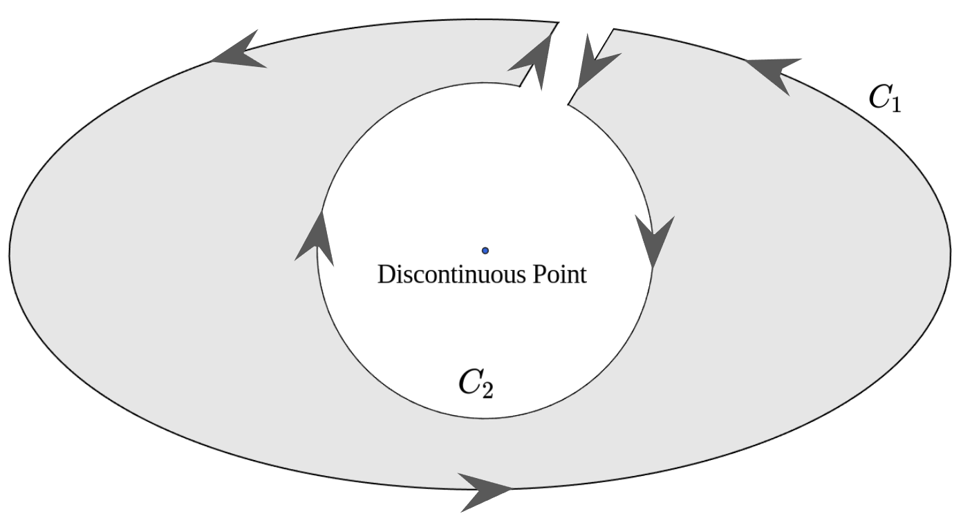
If the integrand contains a discontinuous point, the line integral except for this point in $C$ becomes $0$. Let $C_1$ and $C_2$ be piecewise smooth, not intersecting each other, simple closed curves as above. Then, the line integral except for the discontinuous point is $$\begin{aligned} \oint_C \vec{F} \cdot d\vec{s} = \oint_{C_1} \vec{F} \cdot d\vec{s} + \oint_{C_2} \vec{F} \cdot d\vec{s} = 0 \implies \underbrace{\oint_{C_1} \vec{F} \cdot d\vec{s}}_{\text{counterclockwise}} = - \underbrace{\oint_{C_2} \vec{F} \cdot d\vec{s}}_{\text{clockwise}} \end{aligned}$$

Green’s theorem can be more easily applied if a region containing the discontinuous point is considered as a circle with a radius $1$( or any positive real number).

Application

Example 1. Let $C$ be the circumference of the circle with the radius $1$. Calculate the line integral

$$\begin{aligned} \oint_C (3x^3 + y)dx + (5x + y^5)dy \end{aligned}$$

---

Let $F_1 = 3x^3 + y$ and $F_2 = 5x + y^5$. Then, for the region $R$ surrounded by $C$, $$\begin{aligned} \oint_C (3x^3 + y)dx + (5x + y^5)dy &= \iint_R \left( \cfrac{\partial F_2}{\partial x} - \cfrac{\partial F_1}{\partial y} \right) dy dx = \iint_R (5 - 1)dx dy = 4\pi \end{aligned}$$

Example 2. For $C: \cfrac{x^2}{2} + \cfrac{y^2}{3} = 1$, calculate the line integral

$$\begin{aligned} \oint_C \cfrac{-y dx + x dy}{x^2 + y^2} \end{aligned}$$

---

Note that the integrand has the discontinuous point at $(0, 0)$ which is what $C$ contains as well. Let $C_1$ and $C_2$ be piecewise smooth, not intersecting each other, simple closed curves. Considering $C_2$ containing $(0, 0)$ as a circle with a radius $1$, $C_2$ is given as $X(t) = (\cos t, \sin t)$. $$\begin{aligned} \oint_C \cfrac{-y dx + x dy}{x^2 + y^2} &= -\oint_{C_2} \vec{F} \cdot d\vec{s} = -\int_{C_2} \vec{F}(X(t)) \cdot \left( \cfrac{dx}{dt}, \cfrac{dy}{dt} \right) dt \\ &= - \int_0^{-2\pi} (- \sin t, \cos t) \cdot (-\sin t, \cos t) dt = 2\pi \end{aligned}$$