Gradient, Divergence, Curl, Laplacian

• Overview
• Gradient — Scalar Field to Vector Field
• Divergence — Vector Field to Scalar Field
• Curl — Vector Field to Vector Field
• Laplacian — Scalar Field to Scalar Field

Overview

When a scalar or a vector value is defined at every point in the space, such a mapping, a point to value, is called a field. If a point is mapped to a scalar value, such as temperature or pressure, that is a scalar field. If a point is mapped to a vector, such as wind or ocean current, it becomes a vector field. The most commonly used operations are gradient, divergence, curl, and Laplacian. Gradient and Laplacian operations are mostly applied to scalar field, while the divergence and curl only apply to vector fields. Even though these concepts can be extended to $n$-dimension, consider them only for a point $\mathbf{x} \in \mathbb{R}^3$ here.

Gradient — Scalar Field to Vector Field

The gradient operator measures the rate and direction of change in a scalar field. It is simply a bundle of partial derivatives in all directions, which is perpendicular to the isocontour as mentioned in this note. That is, the gradient operator is denoted by $\nabla$, and for a scalar field $f(\mathbf{x})$, $$\begin{aligned} \nabla f(\mathbf{x}) = \left( \cfrac{\partial f(\mathbf{x})}{\partial x}, \cfrac{\partial f(\mathbf{x})}{\partial y}, \cfrac{\partial f(\mathbf{x})}{\partial z}\right) \end{aligned}$$

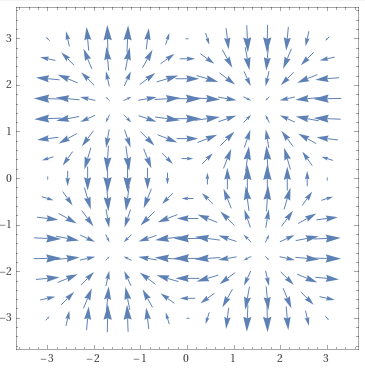
For example, let $f(\mathbf{x}) = \sin x \sin y \sin z$. Then, $$\begin{aligned} \nabla f(\mathbf{x}) = (\cos x \sin y \sin z, \sin x \cos y \sin z, \sin x \sin y \cos z) \end{aligned}$$

A cross-section of this gradient field at $z = \pi / 2$ is shown below.

Divergence — Vector Field to Scalar Field

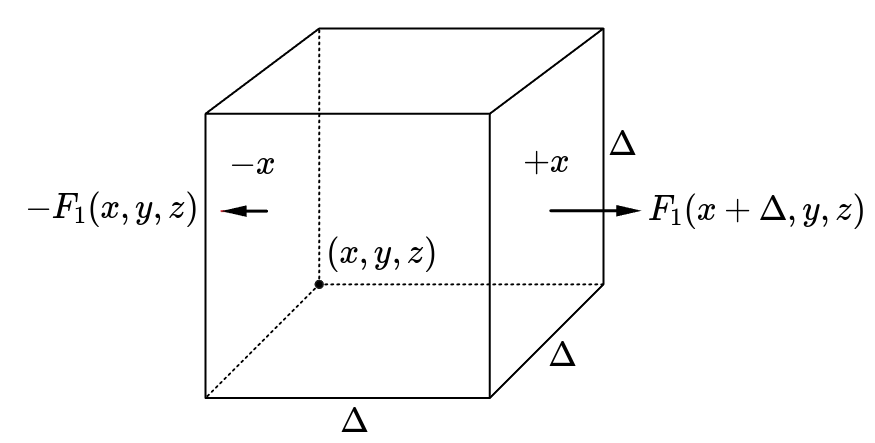
For a given point in a vector field, the divergence operator measures incoming or outgoing flow with a scalar value. This operator can be derived by measuring vectors from a given vector field at each face of a tiny cube with its side length $\Delta$. If the sum of the magnitude of the vectors is greater than zero, then it means some flow is generated inside the cude. If the sum is less than zero, then something is sucking the flow. Let the vector field $F = (F_1, F_2, F_3)$. Since the area of a face is $\Delta^2$, the total amount of stream towards the $x$-direction is, $$\begin{aligned} \Delta^2 F_1(x + \Delta, y, z) - \Delta^2 F_1(x, y, z) \end{aligned}$$

Note that the negative sign is because $+$ means the inward direction in the $-x$ face. Summing these up for every cube face, $$\begin{aligned} &\Delta^2 F_1(x + \Delta, y, z) - \Delta^2 F_1(x, y, z) + \\ &\Delta^2 F_2(x, y + \Delta, z) - \Delta^2 F_2(x, y, z) + \\ &\Delta^2 F_3(x, y, z + \Delta) - \Delta^2 F_3(x, y, z) \end{aligned}$$

This result is the sum of the divergence for the whole volume of the cube. So it should be divided up with the cube’s volume $\Delta^3$. $$\begin{aligned} &\cfrac{F_1(x + \Delta, y, z) - \Delta^2 F_1(x, y, z)}{\Delta} + \\ &\cfrac{F_2(x, y + \Delta, z) - \Delta^2 F_2(x, y, z)}{\Delta} + \\ &\cfrac{F_3(x, y, z + \Delta) - \Delta^2 F_3(x, y, z)}{\Delta} \end{aligned}$$

Therefore, if $\Delta$ approaches $0$, the divergence operator can be derived as follows. $$\begin{aligned} \text{div} F(\mathbf{x}) = \nabla \cdot F(\mathbf{x}) = \left( \cfrac{\partial}{\partial x}, \cfrac{\partial}{\partial y}, \cfrac{\partial}{\partial z} \right) \cdot F(\mathbf{x}) = \cfrac{\partial F_1}{\partial x} + \cfrac{\partial F_2}{\partial y} + \cfrac{\partial F_3}{\partial z} \end{aligned}$$

For example, let $F(\mathbf{x}) = (\sin x \sin y, \sin y \sin z, \sin z \sin x)$. Then, $$\begin{aligned} \nabla \cdot F(\mathbf{x}) = \cos x \sin y + \cos y \sin z + \cos z \sin x \end{aligned}$$

A cross-section of this divergence field at $z = \pi / 2$ is shown below.

Curl — Vector Field to Vector Field

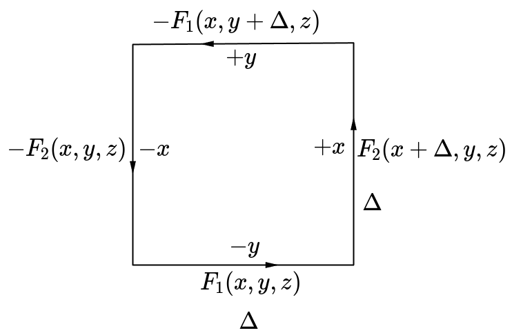
The curl operator evaluates the rotational flow of a vector field at a given point. This operator can be derived by measuring the rotation around a square with its side length $\Delta$. First, for a tiny square in $xy$-plane, the difference of $x$-directional vectors between $+y$ and $-y$ faces is evaluated. Then, the difference between $+x$ and $-x$ faces for $y$-directional vectors is evaluated. Finally, these differences are summed up along the counterclockwise direction. Let the vector field $F = (F_1, F_2, F_3)$. $$\begin{aligned} \left( \cfrac{F_2(x + \Delta, y, z) - F_2(x, y, z)}{\Delta} - \cfrac{F_1(x, y + \Delta, z) - F_1(x, y, z)}{\Delta} \right) k \end{aligned}$$

If $\Delta$ approaches $0$, $$\begin{aligned} \left( \cfrac{\partial F_2}{\partial x} - \cfrac{\partial F_1}{\partial y} \right) k \end{aligned}$$

Since this result measures rotation in the $z$-axis, this evaluation can be extended to $x$- and $y$-axes. $$\begin{aligned} \text{curl} F(\mathbf{x}) = \nabla \times F(\mathbf{x}) = \left( \cfrac{\partial F_3}{\partial y} - \cfrac{\partial F_2}{\partial z}, \; \cfrac{\partial F_1}{\partial z} - \cfrac{\partial F_3}{\partial x}, \; \cfrac{\partial F_2}{\partial x} - \cfrac{\partial F_1}{\partial y} \right) \end{aligned}$$

Note that the direction and the magnitude of the vector correspond to the rotational axis and the amount of the rotation, respectively.

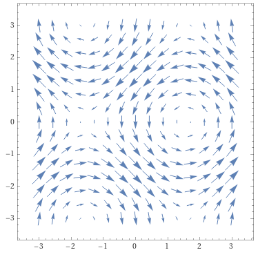
For example, let $F(\mathbf{x}) = (\sin x \sin y, \sin y \sin z, \sin z \sin x)$. Then, $$\begin{aligned} \nabla \times F(\mathbf{x}) = (-\sin y \cos z, -\sin z \cos x, -\sin x \cos y) \end{aligned}$$

A cross-section of this curl field at $z = \pi / 4$ is shown below.

Laplacian — Scalar Field to Scalar Field

The Laplacian operator measures how much the scalar field value at a given location is different from the average field value nearby. In other words, this operator evaluates the bumps on the scalar field. The plane or slope that does not have any curvature has zero Laplacian value. This operator can be explained with the intuitive approach as well.

• The goal is to find the operator that measures how much a scalar field converges or expands.
• Such an operator for a vector field is the divergence.
• However, the divergence operator can accept only a vector field as an input.
• Thus, the idea is to get an intermediate vector field by applying the gradient operator to the original scalar field.
• Now since the input field has become the vector field, the divergence operator can be applied to this field.
• The result scalar field describes the bumpiness of the input field.

$$\begin{aligned} \nabla^2 f(\mathbf{x}) = \nabla \cdot \nabla f(\mathbf{x}) = \cfrac{\partial^2 f(\mathbf{x})}{\partial x^2} + \cfrac{\partial^2 f(\mathbf{x})}{\partial y^2} + \cfrac{\partial^2 f(\mathbf{x})}{\partial z^2} \end{aligned}$$

Since the Laplacian operator measures peaks and edges, one of the popular applications is edge detection for a given scalar field because the output indicates where the edges are and how steep they are. Moreover, if this output is added or subtracted from the original scalar field, it acts like the blur or sharpen effect. Adding the Laplacian field to the original field will lower the sharpest point, thus making the feature point dull and blurry. Exactly the opposite thing happens when subtracting with the Laplacian field, which will sharpen the original.

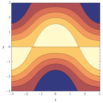
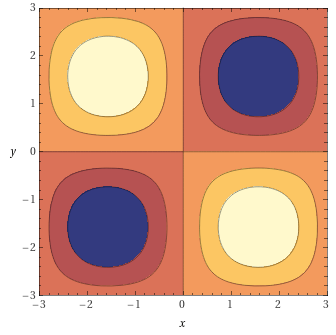
For example, let $f(\mathbf{x}) = \sin x \sin y \sin z$. Then, $$\begin{aligned} \nabla f(\mathbf{x}) = (\cos x \sin y \sin z, \sin x \cos y \sin z, \sin x \sin y \cos z) \implies \nabla^2 f(\mathbf{x}) = -3 \sin x \sin y \sin z \end{aligned}$$

A cross-section of this Laplacian field at $z = \pi / 2$ is shown below.

Reference

[1] Kim, Doyub. (2016). Fluid Engine Development.